Аннотация:
The monitoring of the ionospheric total electron content (TEC) by global navigation satellite system (GNSS) can be a~powerful method to study the interaction of magnetospheric magnetohydrodynamic (MHD) waves with the ionosphere. During the occurrence of intense geomagnetic waves and transients, distinct pulsations with the same periodicity were found in the TEC data from ground-based GNSS receivers. Combined multi-instrument observations, comprising magnetometers, radars, Doppler sounders, aurora imagers, and GNSS receivers, revealed TEC response to various periodic and transient disturbances in the lower part of ultra-low-frequency (ULF) band (periods~1--10~min): toroidal and poloidal Pc4--5 Alfvén waves, compressional mode oscillations, storm sudden commencements (SSCs), and travelling convection vortices (TCVs). However, the effect of TEC modulation by ULF waves is not well examined and a~responsible mechanism has not been firmly identified.

Ключевые слова:
Ionosphere, GNSS, TEC, ULF waves, Pc5 pulsations, TCV, SSC, MHD waves

1 Introduction

The ionosphere represents the inner boundary of the near-Earth environment where the energy exchange occurs between the atmosphere and outer space plasma. Ultra-low frequency (ULF) waves are a ubiquitous carrier of energy in geospace [Lin et al., 2025]. Magnetohydrodynamic (MHD) waves provide an effective channel of energy transfer from the outer magnetosphere to the lower ionosphere, and eventually to the ground. The interaction between the solar wind and magnetosphere acts as a permanent driver of various types of MHD waves in the ULF band that fill the entire magnetosphere and reach its inner boundary, the ionosphere. While ground magnetometers and magnetospheric satellites provide tremendous amounts of information about ULF wave properties in the magnetosphere and on the Earth, the wave properties in the ionosphere remain unavailable to in-situ observations. Low-Earth orbit (LEO) satellites can detect only a high-frequency part of ULF spectrum (Pc1–3 pulsations, periods \(T = 0.2\)–45 s), because a satellite remains in a region occupied by these waves during at least several periods. Signatures of long-period waves (Pc4–5, Pi2–3 with \(T > 1\) min) look like quasi-static structures in LEO satellite observations. Ionospheric signatures of such long-period waves can be detected by modern radio sounding techniques: Doppler sounders [Menk et al., 2007; Pilipenko et al., 2013; Waters et al., 2007], coherent scatter high-frequency (HF) radars [Gjerloev et al., 2007; Lester et al., 2000; Ponomarenko et al., 2001; Teramoto et al., 2014], and VHF European Incoherent Scatter (EISCAT) radar facility [Crowley et al., 1985; Hazendonk et al., 2024; Lathuillere et al., 1986; Wright et al., 1998]. ULF waves are the most powerful wave processes in the terrestrial environment, and they can significantly modulate the ionospheric plasma. The radar community has demonstrated that ULF pulsations in the nominal Pc5/Pi3 band (2–10 min periods) can significantly modulate the ionosphere, including the ionospheric electric field \(\mathbf {E}\) and plasma convection velocity \(\mathbf {V}\) [Norouzi-Sedeh et al., 2015; Sakaguchi et al., 2012]; field-aligned current [Fenrich et al., 2006]; E-layer electron density and ionospheric conductance [Belakhovsky et al., 2016; Buchert et al., 1999]; electron and ion temperatures in both F and E layers [Pilipenko et al., 2014a]. The effects of the ionospheric modulation by ULF waves and transients were found at all latitudes, from low latitudes up to the polar cap [Alfonsi et al., 2022; Bland and McDonald, 2016; Shi et al., 2018].

The ever-growing array of four main global navigation satellite systems (GNSS), such as GPS, GLONASS, Beidou, and Galileo, provides information on variations of a radio-path-integrated ionospheric parameter — the total electron content (TEC). Early results, during the era of Faraday technique with geostationary beacons, reported TEC fluctuations related to geomagnetic variations in the Pc4 range (\(T = 30\)–50 s) [Davies and Hartmann, 1976; Okuzawa and Davies, 1981]. Nowadays, the GNSS technique makes it possible to detect an ionospheric image of catastrophic events in the upper atmosphere [Astafyeva and Shults, 2019; Yasyukevich et al., 2024]. TEC observations with world-wide array of GNSS receivers have become a powerful tool to monitor the ionospheric disturbances caused by acoustic-gravity waves originated from impulsive events below the ionosphere [Afraimovich et al., 2013; Astafyeva, 2019; Huang et al., 2019; Komjathy et al., 2012; Meng et al., 2019], including earthquakes, tsunamis, volcanic eruptions, explosions [Galvan et al., 2011; Shalimov et al., 2019; Tsai et al., 2011; Vesnin et al., 2023].

The GNSS/TEC technique has turned out to be sensitive enough to detect ionospheric signatures of long-period ULF waves and transients as well. Information on the GNSS-derived TEC can provide a new insight into the physics of the MHD wave interaction with the ionospheric plasma. Recent event-based studies (dispersed in the literature) that have used the GNSS/TEC data are summarized in this review. Possible mechanisms of TEC modulation by MHD waves will be discussed elsewhere.

2 Methodology of GNSS Measurements with Simultaneous Magnetometer, Radar, and Riometer Observations

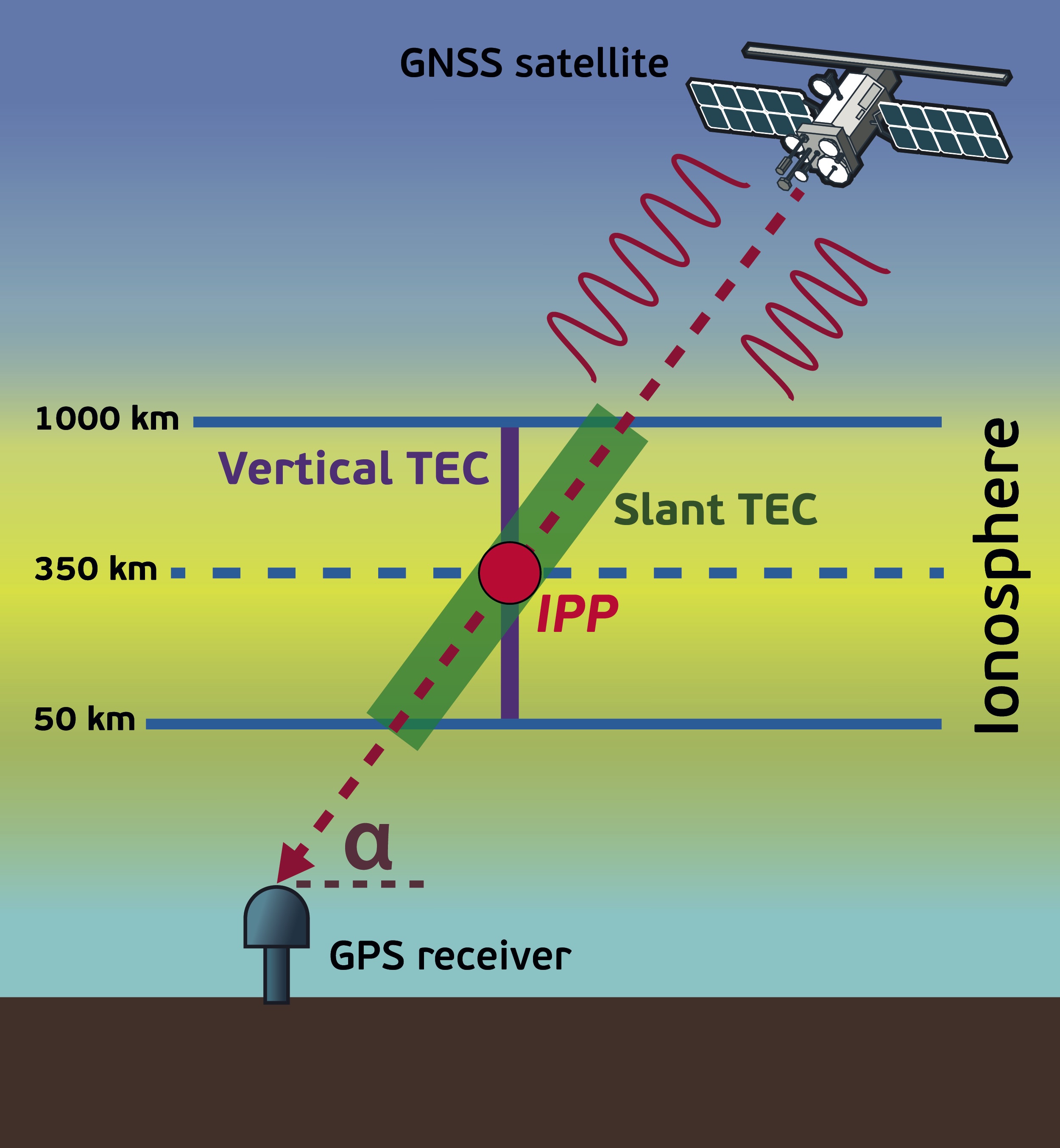
Dual-frequency method uses the phase information from radio signals transmitted from GNSS satellites at the L1 (1575.42 MHz) and L2 (1227.60 MHz) frequencies for estimating the slant TEC. The slant TEC along a radio path can be converted into the vertical vTEC, denoted here as \(N_{\mathrm {T}}\), by assuming a fixed altitude of pierce point (PP). A schematic illustration of the GNSS/TEC technique is shown in Figure 1. As a measure of columnar density \(N_{\mathrm {T}}\), the TEC unit (1 TECu = 10\(^{16}\) m\(^{-2}\)) is used. GPS dual-frequency phase measurements are freely available as daily data files in RINEX format from the International GNSS Service portal (https://igs.org, ftp://cddis.gsfc.nasa.gov). Most ULF studies used the standard TEC data with 30 s resolution from an array of GPS receivers. Higher resolution, like 1-second, TEC data has been used in recent studies [Hartinger et al., 2025; Shen et al., 2024].

The TEC data are augmented by magnetometer data from the world-wide array with sampling period 1 s or 1 min. The energetic (\(> 30\) keV) electron precipitation into the lower ionosphere can be monitored with vertical or multi-beam riometers that measure cosmic noise absorption. During night-time hours, the precipitation of soft electrons (1–10 eV) can be controlled with auroral imagers in the oxygen red (630.0 nm) and green (557.7 nm) optical emissions.

Observations of ionospheric flow vectors in the E and F regions of the ionosphere over a wide latitudinal and longitudinal area with a high temporal and spatial resolution became possible with a global network of over 30 Super Dual Auroral Radar Network (SuperDARN) radars. Each radar scans through 16 beams with an azimuthal separation 3.24\(^\circ \) resulting in a full scan once every 1–2 min. Each beam is divided into 75 range gates with 45 km range resolution. The radars detect coherent backscatter from electron density irregularities and measure Doppler velocity \(\mathbf {V}\) along a beam which corresponds to the \(\mathbf {E} \times \mathbf {B}_{0}\) drift. ULF wave signatures are identified in the radar data as periodic fluctuations in the Doppler velocity which are superposed on the background convection flow. SuperDARN radars became a valuable tool, providing information about ULF wave latitudinal structure and azimuthal propagation characteristics [Fenrich et al., 2006; Ponomarenko et al., 2001; Ziesolleck et al., 1998].

The altitudinal profile of the ionospheric plasma drift velocity \(\mathbf {V}\) and corresponding electric field \(\mathbf {E}\) with 30 s cadence can be obtained using UHF EISCAT radar. The EISCAT system also measures the altitude profile up to ~400 km of electron density \(N_{\mathrm {e}}(z)\), ion \(T_{\mathrm {i}}(z)\) and electron \(T_{\mathrm {e}}(z)\) temperatures along a beam aligned with the geomagnetic field \(\mathbf {B}_{0}\). The EISCAT facility comprises receivers at Sodankyla (SOD) and Kiruna (KIR), and receiver-transmitter at Tromso (TRO). Intersection of receiving paths from SOD and KIR at altitude ~290 km is located nearly above the magnetic station TRO.

3 Examples of TEC Modulation by Various Types of ULF Waves and Responsible Mechanisms

The interaction between the solar wind and magnetosphere provides a rich source for various types of ULF disturbances in the Pc4–5 band (\(T \approx 1\)–10 min). Here we present examples of the TEC response to different types of ULF waves and transients.

3.1 Magnetosphere Compression by Interplanetary Shock

A rapid displacement of the magnetopause caused by an interplanetary shock induces a magnetic disturbance propagating as a fast compressional wave inward the magnetosphere. Most of this wave energy is scattered throughout the magnetosphere, but some reaches the Earth. The global response to the interplanetary shock is observed on the ground as storm sudden commencement (SSC) impulse. The positive main impulse (MI) of SSC is gradually built up over time, governed by the propagation time of MHD disturbance from different parts of the magnetopause and the time of sweeping the dayside magnetosphere by a shock. At the front of a fast compressional wave an Alfvén pulse can be generated. This pulse was suggested to give rise to a negative preliminary impulse (PI) preceding a MI. Thus, the MI and PI are two nearly-overlapping wave processes of different physical nature.

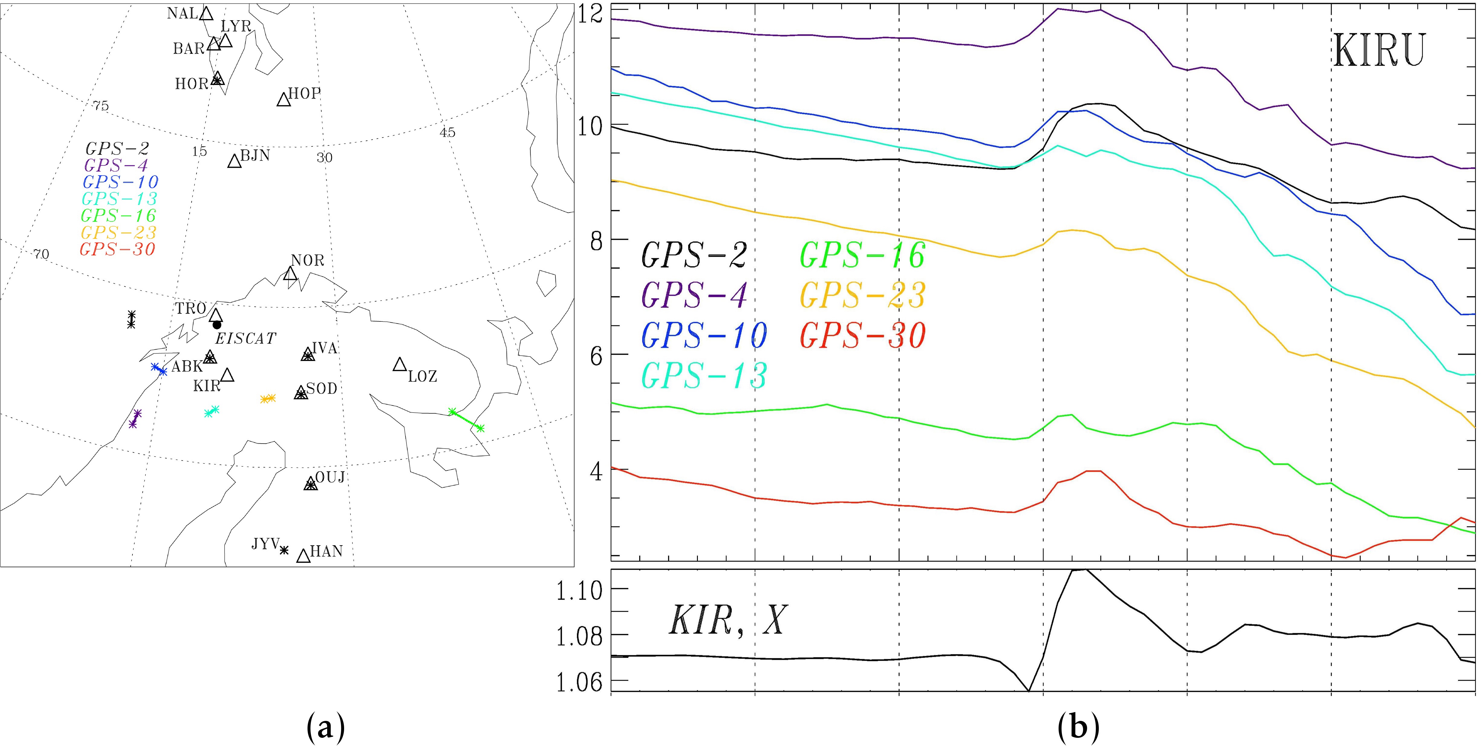
In [Pilipenko et al., 2018] a multi-instrument study of the ionospheric response to the arrival of a shock on Jan. 24, 2012, was performed. At ~15:00 UTC the shock was recorded as a rapid jump of the solar wind velocity from ~400 km/s up to ~700 km/s, an increase in the interplanetary magnetic field magnitude from ~3 nT up to ~30 nT, and an enhancement of the solar wind density and dynamic pressure up to ~15 cm\(^{-3}\) and ~10 nPa. The map with locations of magnetic stations, riometers, optical imagers, and GPS receivers during this event is shown in Figure 2a.

Detailed comparison of riometer absorption and geomagnetic variations in the morning and post-noon sectors demonstrated that the onset of energetic electron precipitation responsible for the riometer burst nearly coincided with the onset of PI and was ~1 min ahead of the MI.

In the evening sector, at a background of gradual increase of vTEC, a superposed positive pulse of vTEC was observed with an amplitude up to ~1 TECu, and a relative increase of ~8–9% (Figure 2b). The onset of the TEC pulse coincided with the PI, but no PI signatures were seen in the TEC waveforms. The peak of the TEC pulse coincided with the peak of geomagnetic MI.

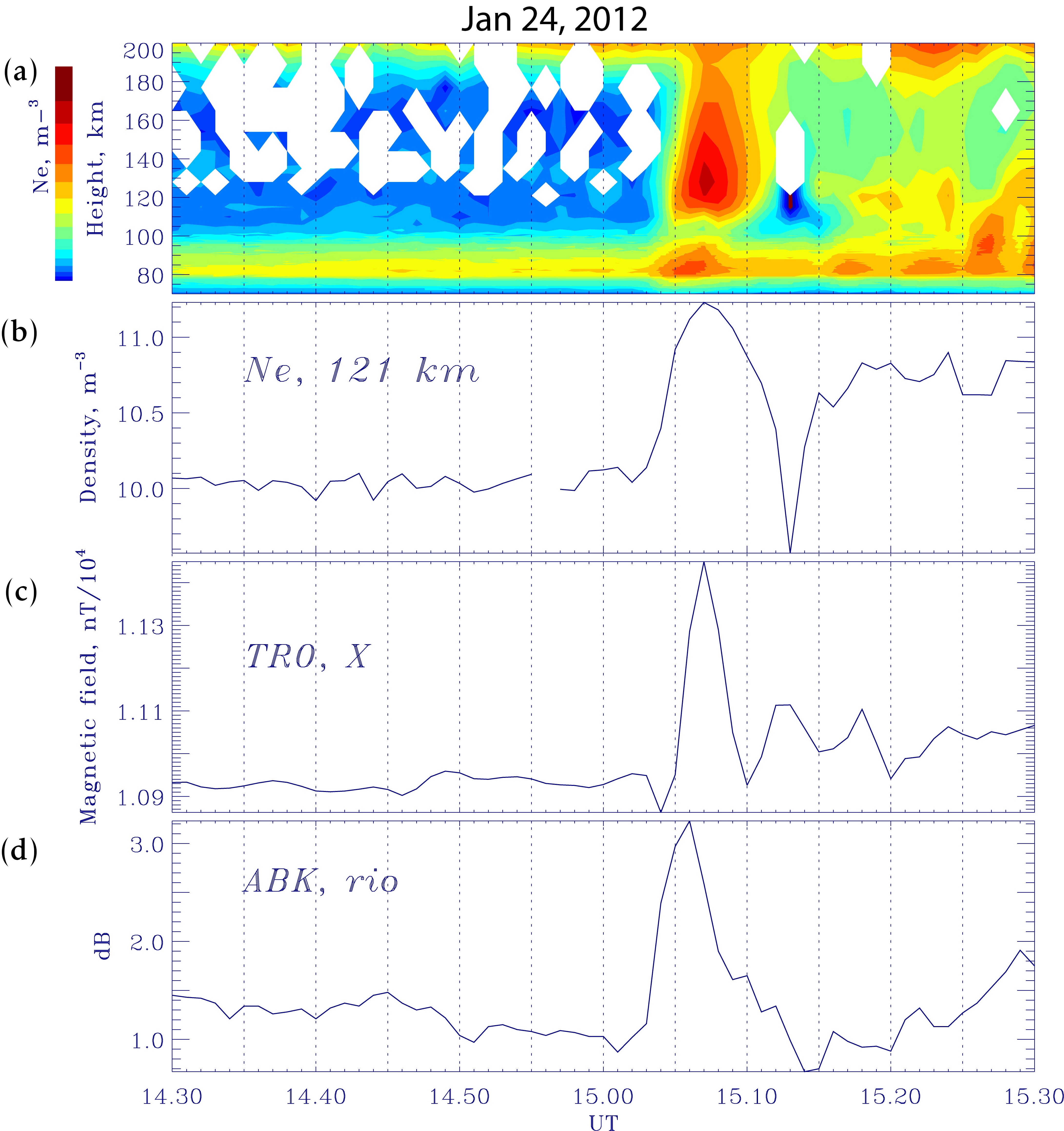
To identify the mechanism responsible for the observed ionospheric response, it is important to determine the vertical structure of an ionospheric disturbance. Such a structure was measured with the EISCAT radar [Belakhovsky et al., 2017b]. The most evident response in the electron density \(N_{\mathrm {e}}\) was seen at altitudes 100–180 km (Figure 3). A growth of \(N_{\mathrm {e}}\) in the E layer (120 km) started simultaneously with the riometer increase and PI. The increase of \(N_{\mathrm {e}}\) reached its maximum simultaneously with the MI peak. The onset and duration of the EISCAT-measured \(N_{\mathrm {e}}\) pulse and the GPS-detected TEC pulse were nearly the same, 15:04–15:11 UTC, which indicated that both pulses were manifestations of the same disturbance.

The precipitation of energetic electrons and ionization of the lower ionosphere during SSC, responsible for a disturbance recorded by riometers, can influence only the bottom E and D layers. However, the contribution of these layers into TEC is small as compared with that of the F layer. The mechanisms responsible for the modulation of the ionospheric plasma upon the interaction of an incident MHD pulse with the ionosphere-atmosphere-ground system may include plasma compression. The relative amplitude of plasma compression is to be comparable to the relative change of the magnetic field, i.e., \(\Delta N_{\mathrm {e}}/N_{\mathrm {e}} \approx \Delta B/B\). According to this mechanism, the lack of \(N_{\mathrm {e}}\) response in the F layer evidenced by the EISCAT observations is hard to comprehend. During the SSC event under study, a shock-associated aurora was observed by a ground photometer. The 1–10 keV electrons responsible for this aurora are absorbed and ionize the ionospheric plasma at an altitude of 110–160 km. This altitude range corresponds well to the ionospheric density enhancement detected by EISCAT. Therefore, the precipitation of soft electrons caused by the shock compression may be responsible for the SSC-associated TEC pulse. A nearly simultaneous response in riometer, TEC, and EISCAT may be interpreted as a SSC-stimulated precipitation of electrons with a wide energy range, from soft (\(\leq \) keV) to energetic (tens of keV).

3.2 Compressional Waveguide Mode

During the recovery phase of the 31 October 2003 storm very intense (up to several hundred nT) global Pc5 waves were observed. During this event coherent quasi-monochromatic variations were observed over a wide range of latitudes down to the near-equatorial latitudes [Potapov et al., 2011]. Pc5 waves at very low latitudes cannot be associated with Alfvénic mode but are probably the manifestation of compressional wave associated with the magnetospheric cavity or waveguide modes [Marin et al., 2014].

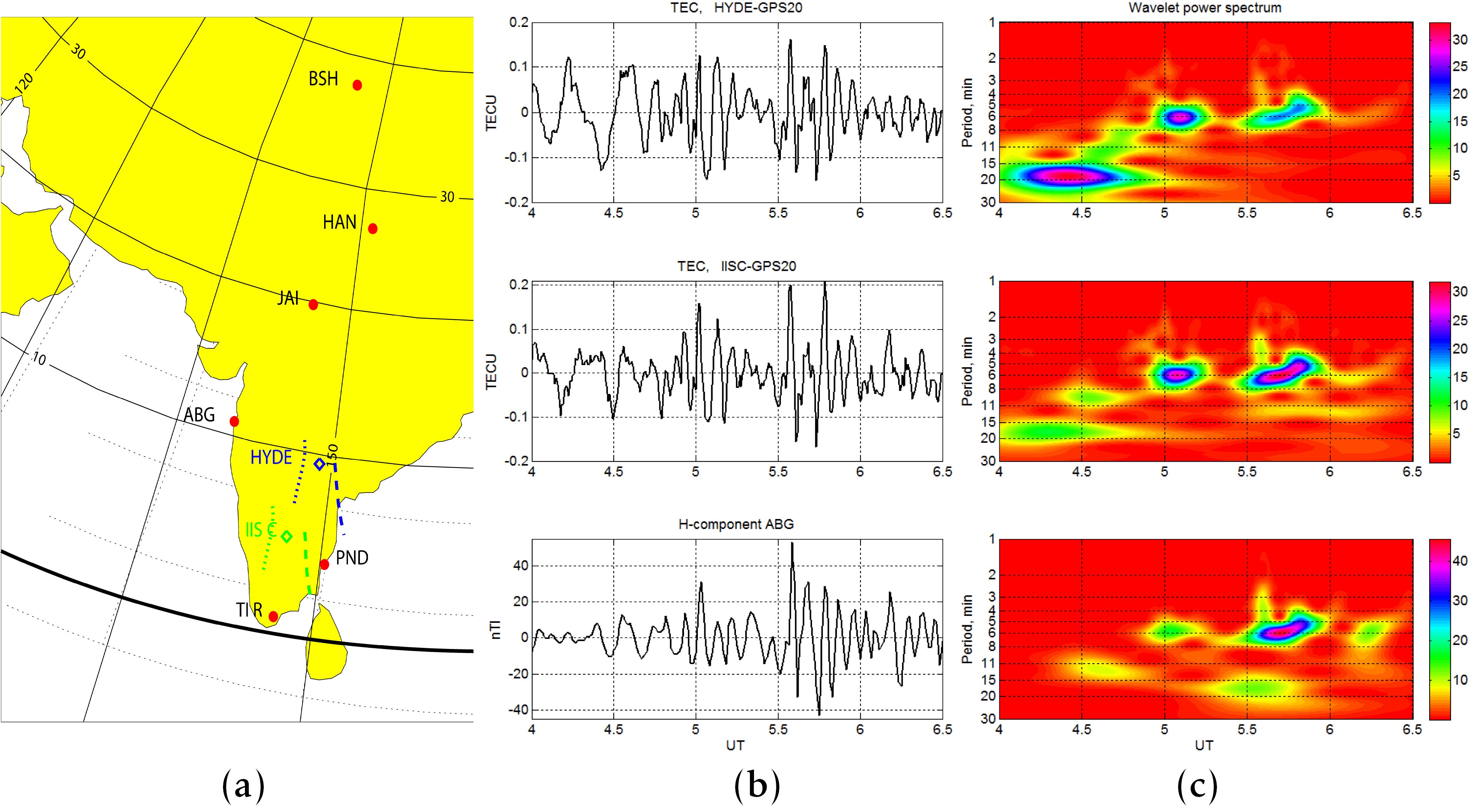
During intervals of enhanced global Pc5 activity, TEC fluctuations from the GPS receivers HYDE and IISC in the Indian sector were compared with geomagnetic variations (Figure 4a) by [Vorontsova et al., 2016]. During the time interval 04:00–06:30 UTC TEC fluctuations along the HYDE-GPS20 and IISC-GPS20 radio paths had nearly the same periodicity as geomagnetic pulsations (Figure 4b). Wavelet analysis showed similar wave disturbances in TEC and geomagnetic field variations having periodicity ~4–6 mins. The peak-to-peak amplitudes of TEC and magnetic pulsations were \(\Delta N_{\mathrm {T}} \approx 0.2\) TECu and \(\Delta H~\approx 50\) nT, respectively. Cross-spectral analysis confirmed a good correspondence between TEC and magnetic field variations (cross-coherence \(\gamma \approx 0.8\)) and indicated that geomagnetic pulsations in \(H\) component were almost in-phase with TEC fluctuations.

Thus, TEC modulation at low latitudes may be related to plasma compression in MHD mode with a significant compressional component. The plasma oscillations in the fast magnetosonic mode are to be of about the same relative amplitude as magnetic field oscillations, that is \(\Delta N_{\mathrm {T}}/N_{\mathrm {T}} \approx \Delta N/N \approx \Delta B/B\). Assuming that in the F layer \(B_{0} = 25000\) nT, and \(N_{\mathrm {T}} = 40\) TECu, the 50 nT geomagnetic pulsations can produce ~0.2% modulation of geomagnetic field and TEC. This value is just half of the observed TEC modulation of ~0.4% and does not contradict the proposed mechanism.

3.3 Toroidal Large-Scale Alfvén Mode

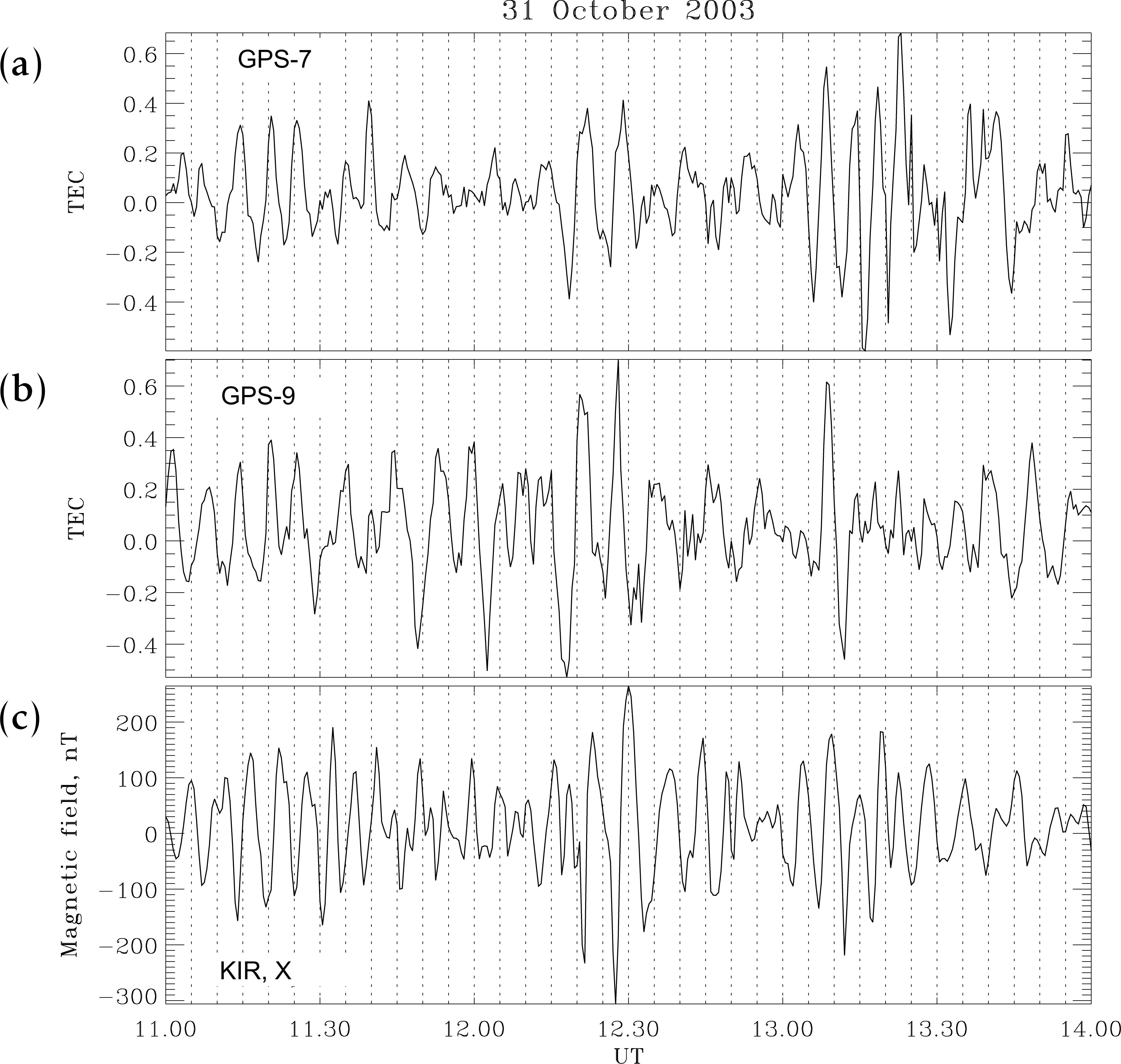
An intriguing effect of TEC modulation by intense Pc5 pulsations was found by [Pilipenko et al., 2014b] at sub-auroral latitudes during the strong magnetic storm on 31 October 2003 (Figure 5a). During the recovery phase of this storm very intense quasi-monochromatic ~2.5 mHz Pc5 waves were observed over a wide range of geomagnetic latitudes, from ~70\(^\circ \) to ~50\(^\circ \). During the period with elevated geomagnetic ULF activity, detrended TEC data showed the occurrence of persistent TEC periodic oscillations nearly on the same time scale as geomagnetic pulsations (Figure 6). The cross-spectral analysis showed a high coherence (\(\gamma \approx 0.9\)) between the periodic geomagnetic and TEC variations. Moreover, both geomagnetic pulsations and TEC variations demonstrated westward propagation, but with somewhat different azimuthal wave numbers \(m\), ~0.9 and ~0.5 respectively (Figure 5b). The observed effect seems puzzling because Pc5 pulsations are associated with Alfvén waves, which are known to be a non-compressional mode. Similar periodic TEC responses to Alfvén oscillations, but in other frequency bands, were also observed for Pc4 pulsations [Watson et al., 2016] and Pc6 pulsations [Watson et al., 2015].

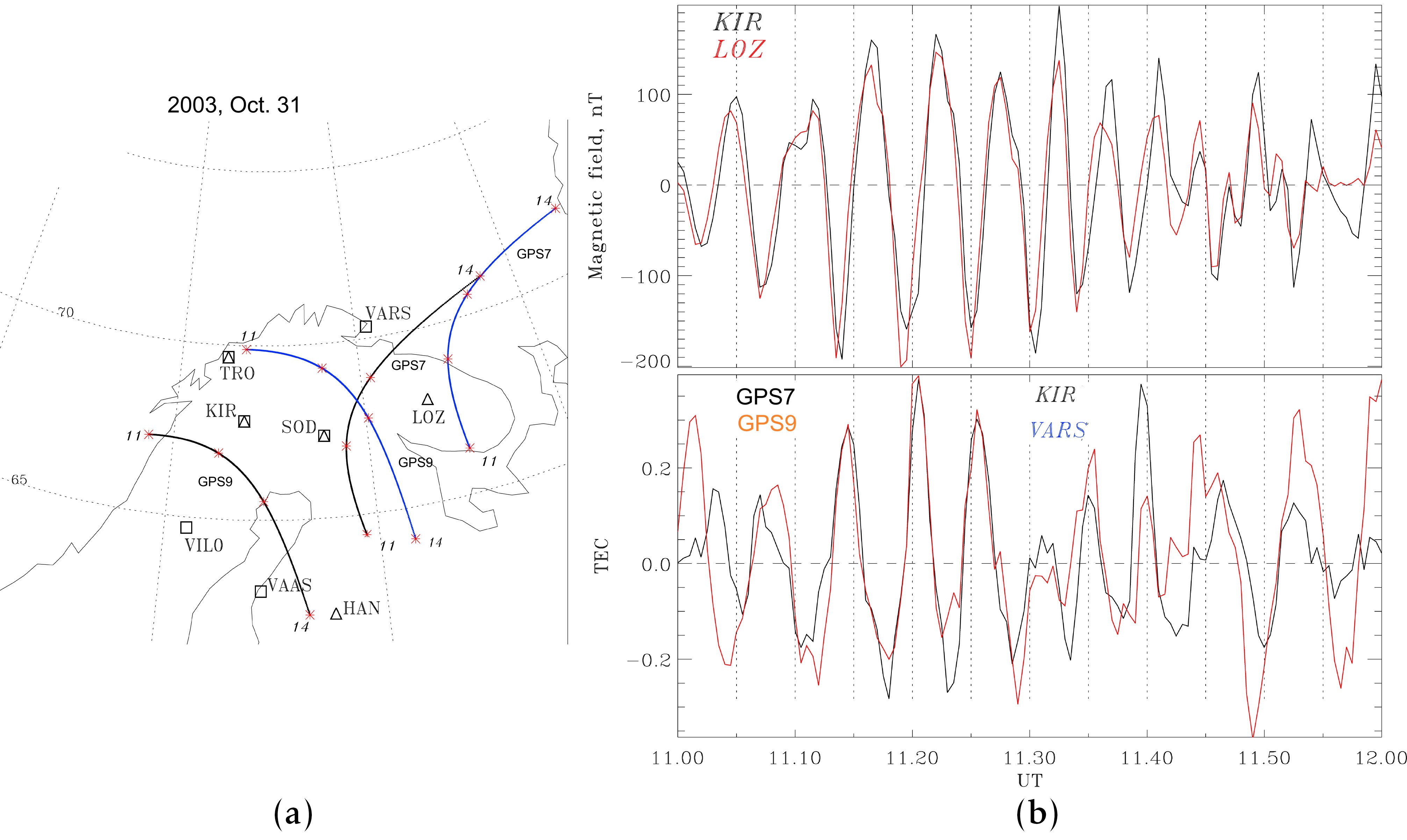
The peak-to-peak amplitudes of ionospheric plasma oscillations were \(\Delta N_{\mathrm {T}} \approx 0.6\)–2.0 TECu, and those of magnetic pulsations were \(\Delta B \approx 400\) nT. The ratio between the spectral densities of \(\Delta N_{\mathrm {T}}\) and \(\Delta B\) variations at central frequency was \(\Delta N_{\mathrm {T}}/\Delta B \approx 2.10\)–3 TECu/nT. In the Pc5 event under consideration \(N_{\mathrm {T}} \approx 40\) TECu, \(\Delta N_{\mathrm {T}} \approx 1\) TECu, hence \(\Delta N_{\mathrm {T}}/N_{\mathrm {T}} \approx 2.5\%\). At the same time, the relative amplitudes of magnetic pulsations were \(\Delta B/B_{0} \approx 1\%\). Thus, during this event, the depth of TEC variations is ~2–3 times larger than that of magnetic pulsations, though one may expect the wave-induced fractional variations of plasma and magnetic field to be of the same magnitude, as in any linear wave. As a shear Alfvén wave does not produce plasma/magnetic field compression, any compressional effects can arise only upon interaction of this mode with the anisotropic inhomogeneous ionosphere. In principle, ULF modulation of energetic electron precipitation, inducing an additional periodic ionization of the lower ionosphere, can cause periodic TEC variations with much higher depth than geomagnetic field variations. However, during the event under consideration no periodic electron precipitation occurred, as evidenced by simultaneous riometer observations. The mechanism of the field-aligned plasma transport by Alfvén wave can theoretically produce relative amplitudes of TEC variations larger than that of geomagnetic pulsations.

3.4 Alfvén Wave Impact on the Ionosphere as Observed by EISCAT

Possible mechanisms of TEC modulation by magnetospheric ULF waves may provide main contribution either to the upper ionosphere (F layer) or to the lower ionosphere (E layer and bottom of F layer). The ability of EISCAT to reveal the contribution of ionospheric plasma density oscillations at different altitudes to the total TEC fluctuations may help to identify a responsible mechanism. The vertical structure of the electron density oscillations can be also examined with Poker Flat Incoherent Scatter Radar (PFISR) [Wang et al., 2020].

During the 31 October 2003 event with elevated Pc5 activity, TEC fluctuations were compared with ground geomagnetic variations and ionospheric parameters determined by EISCAT radar [Belakhovsky et al., 2016]. TEC data showed gradual variations with superposed small-scale fluctuations. After detrending, quasi-periodic TEC pulsations have been revealed over a wide latitudinal range [Pilipenko et al., 2014a]. TEC fluctuations, magnetic variations, and EISCAT-derived ionospheric density \(N_{\mathrm {e}}\) in the lower ionosphere and ion temperature \(T_{\mathrm {i}}\) showed the occurrence of persistent periodicity in all these parameters (Figure 7). The peak-to-peak amplitudes of TEC oscillations are \(\Delta N_{\mathrm {T}} \approx 0.6\)–1.0 TECu, and those of magnetic pulsations are \(\Delta B \approx 400\) nT (\(X\) component). At the same time, the riometer data did not demonstrate periodicity similar to magnetometer data. Spectral analysis confirmed the occurrence of the same periodicity with \(f \approx 2.4\) mHz in variations of the geomagnetic field, TEC, and EISCAT \(N_{\mathrm {e}}\).

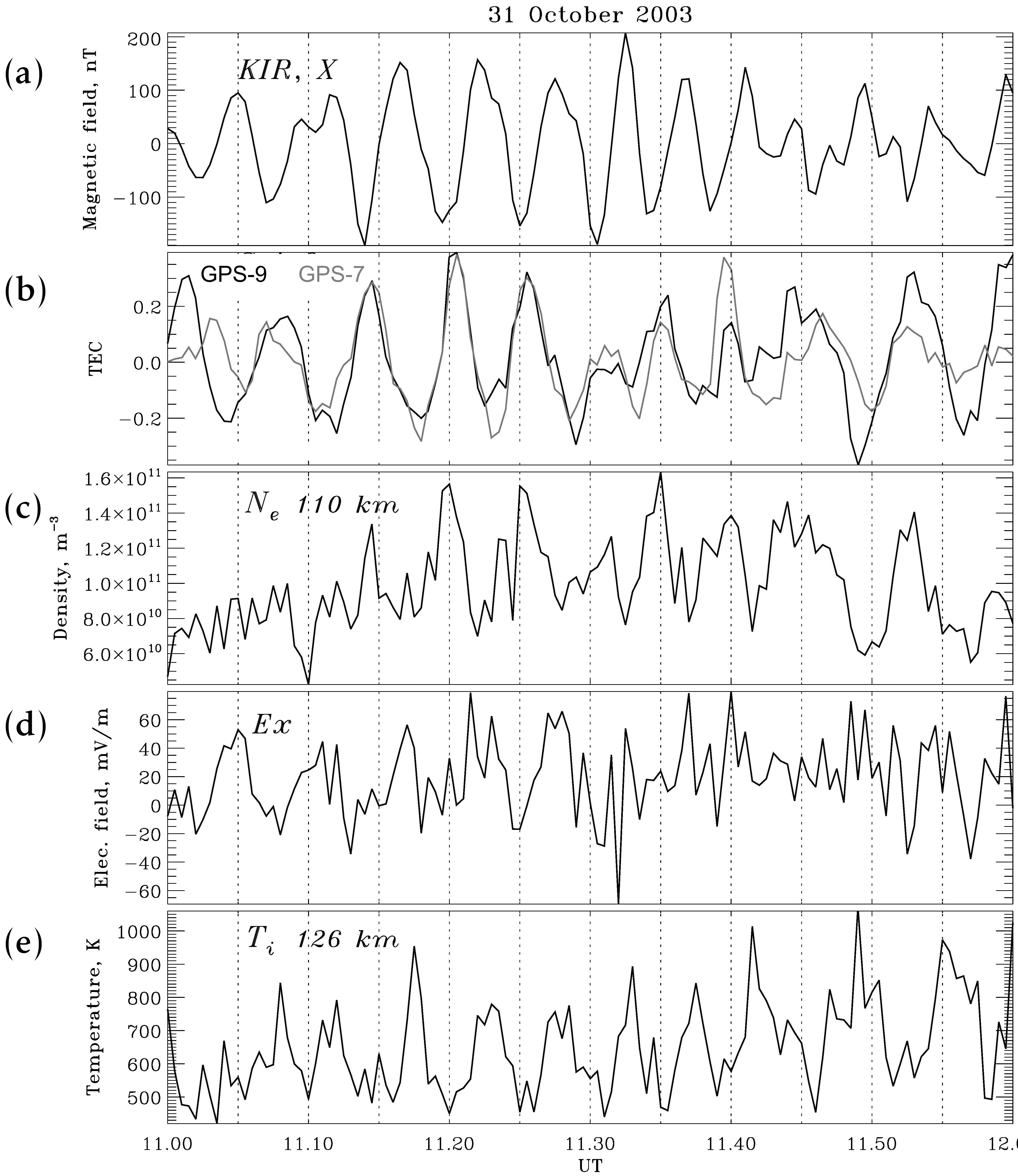
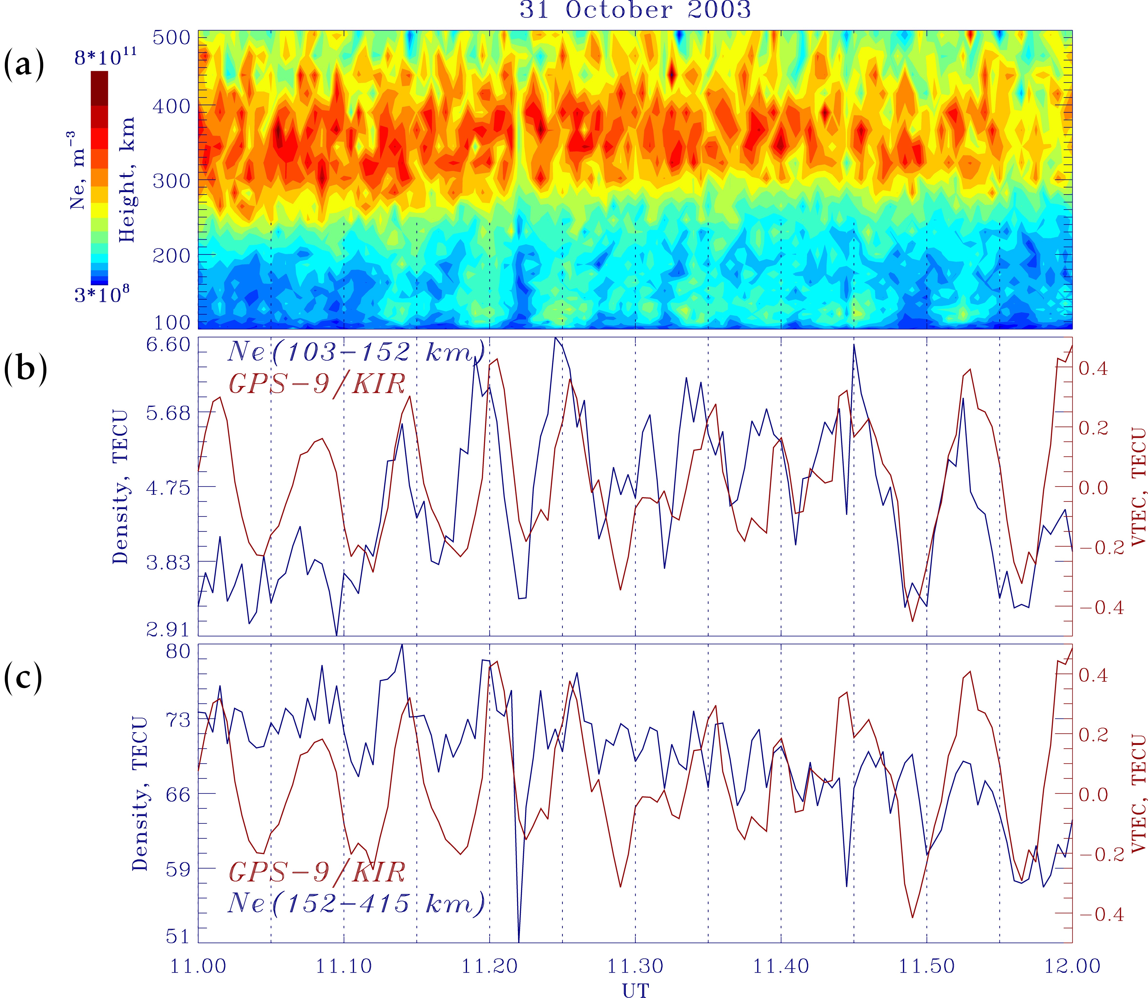
To find out which altitudes contribute most to the TEC variations, the ionospheric \(N_{\mathrm {e}}(z)\) data from EISCAT have been integrated over two different altitude ranges: the bottom ionosphere from 103 km to 152 km; and the F layer from 152 km to 415 km (Figure 8). The height-time diagram of \(N_{\mathrm {e}}(t)\) variations and altitude-integrated ionospheric densities \(\langle N_{\mathrm {e}} \rangle \) were compared with actual TEC variations. This comparison showed that the main contribution was provided by lower ionosphere, up to ~150 km (that is the E layer and lower F layer).

The field-aligned current and flux transported by an Alfvén wave incident onto the ionosphere cause an additional accumulation of plasma in regions with strong vertical gradients of the plasma density profile \(N_{\mathrm {e}}(z)\). A significant part of an Alfvénic current is transported by a background suprathermal electron flux into the ionosphere. These electrons do not ionize the ionospheric plasma additionally, so they cannot be detected by riometers, but they can pump the ionospheric TEC. As a result, the plasma density in the lower ionosphere may increase. The EISCAT-observed increase of \(N_{\mathrm {e}}\) at altitudes 110–180 km is in accordance with this mechanism.

3.5 Periodic Modulation of the Upper Ionosphere by Alfvén Waves as Observed by SuperDARN Radars and GNSS/TEC Technique

During the Pc5 wave event on 2 March 2002 simultaneous observations by magnetometers, GNSS receivers, and SuperDARN radars at King Salmon (KSR) and Kodiak (KOD) sites were compared (Figure 9) [Kozyreva et al., 2020]. The beam KSR/03, corresponding to the azimuthal direction, evidenced that the ionospheric proxy of Pc5 waves propagated anti-sunward with the wave number \(m = 8 \pm 3\) (Figure 10a). The beam KOD/04 corresponded to the meridional direction, and the Range-Time-Intensity plot from beam 6 indicated the apparent poleward wave propagation (Figure 10b).

Despite a rather low amplitude of geomagnetic Pc5 pulsations, ~15–20 nT, TEC response was evident. A comparison of waveforms of Doppler radar velocity, Rate-Of-TEC change (ROT) from two nearby radio paths and magnetic field confirmed a correspondence between Pc5 signatures in all instruments. The KOD/04 radar velocity (corresponding to the north-south \(V_{x}\) component) data showed burst of Pc5 waves at ~15:30 UTC with peak-to-peak amplitude ~300 m/s. A comparison of KOD/10 radar Doppler velocity, ROT from INVK/GPS23 track and magnetic field (\(X\) component) from DAW magnetometer confirmed a good correspondence between Pc5 signatures in all instruments (Figure 11a). Beam KOD/GPS10 went across the PP of radio path INVK/23, and DAW is far from the PP, but at the same geomagnetic latitude. Spectra of both ionospheric and magnetic field variations confirmed the occurrence of coherent Pc5 pulsations (Figure 11b).

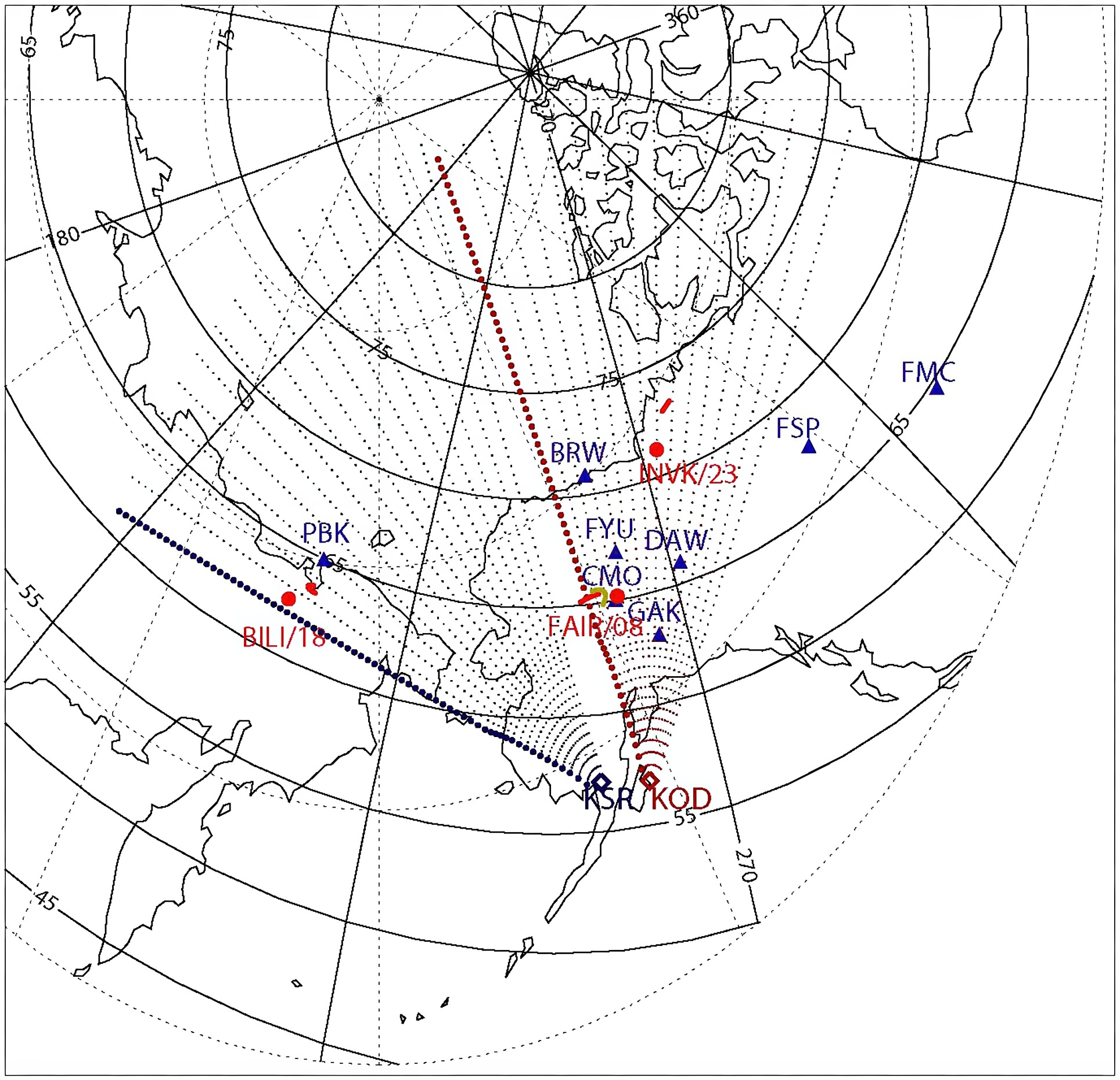
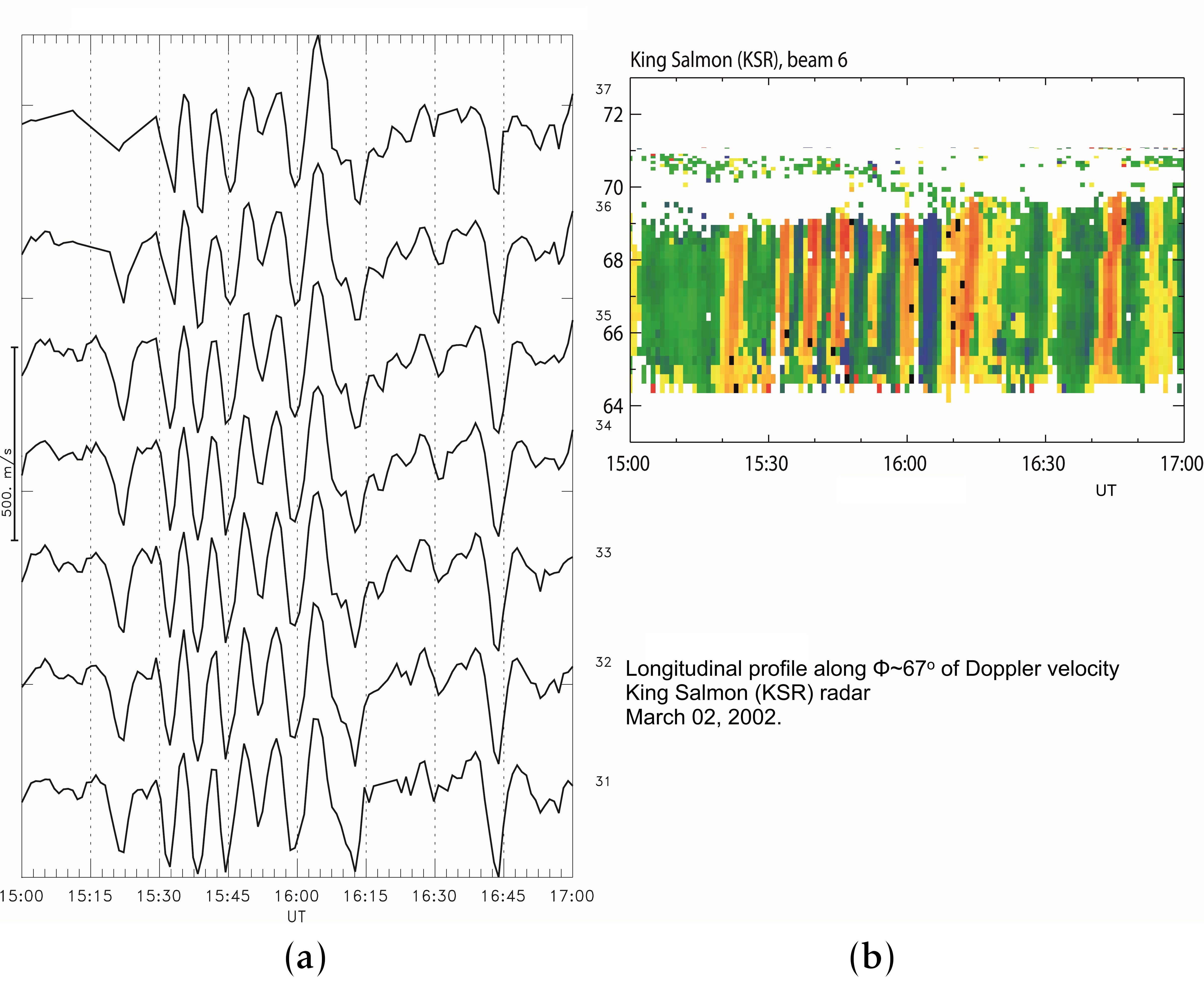
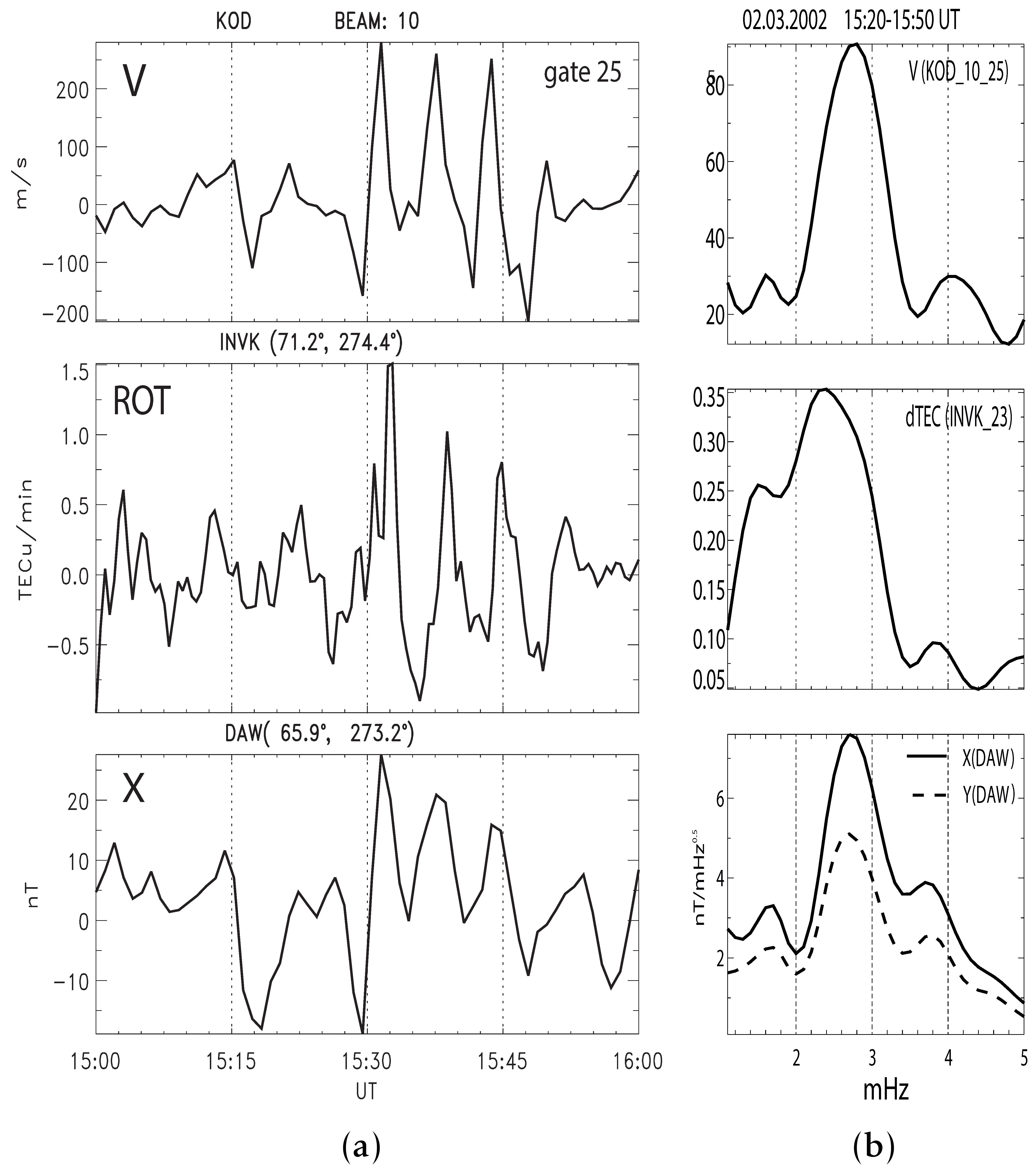
The ratio between Doppler \(\mathbf {V}\) and magnetic \(\mathbf {B}\) pulsations varied widely depending on the selected instrument pair. At central frequency 2.6 mHz this ratio for KOD radar was on average \(V_{x}/X(\mathrm {CMO}) \approx 7\) (m/s)/nT; and \(V_{x}/X(\mathrm {DAW}) \approx 12\) (m/s)/nT. The ratio of spectral densities between pulsations of the ROT and ionospheric velocity also varied in a wide range depending on selected instruments. On average this ratio was \(\mathrm {ROT}(\mathrm {FAIR/GPS08})/V_{x}(\mathrm {KOD/GPS04}) \approx 7.6 \cdot 10^{-4}\) (TECu/min)/(m/s). The amplitude relationships derived from coordinated SuperDARN and GNSS/TEC observations provide valuable information for modelers trying to interpret the effects of the ULF wave modulation of the ionosphere [Shinbori et al., 2024].

3.6 TEC and Aurora

Geomagnetic ULF pulsations were found to be accompanied by simultaneous pulsations both in TEC and in auroral intensity. As an example, [Belakhovsky et al., 2017a] examined Pc5 pulsations with amplitude ~300 nT in the morning sector at the Canadian Array for Realtime Investigations of Magnetic Activity (CARISMA) network stations. At the geostationary GOES-8 satellite these oscillations had a toroidal polarization. According to the data from longitudinally separated stations GILL-PBQ, the azimuthal wave number was estimated to be \(m \approx 2.7\)–4.0 for the observed Pc5 pulsations. Such a value of \(m\) really corresponds to the large-scale azimuthal structure of geomagnetic oscillations, i.e. the toroidal Alfvén mode propagating in the antisolar direction.

Geomagnetic Pc5 oscillations were accompanied by simultaneous pulsations in the intensity of auroral emissions of oxygen (557.7, 630.0 nm) and nitrogen (471 nm) according to the data from meridional scanning Northern Solar Terrestrial Array (NORSTAR) photometers. Similar oscillations were seen in TEC and in the riometric absorption. Auroral Pc5 pulsations reflected the resonant structure of the simultaneously observed toroidal geomagnetic Pc5 pulsations. A characteristic structure of auroral Pc5 pulsations was that each brightness element was tilted to the right, which corresponded to the arrival of particles causing the luminosity brightening first at lower and then at higher latitudes, similar to geomagnetic Pc5 pulsations. The apparent propagation from lower to higher latitudes is a reflection of the phase structure of the field-aligned currents carried by a wave in the Alfvén resonance region. Similar Pc5 pulsations were also recorded in the ionospheric TEC. Spectral analysis showed a coincidence of maxima at frequencies 3.0, 3.8 mHz for pulsations in the magnetic field, auroral intensity, riometric absorption, and ionospheric TEC.

The presence of a high correlation between Pc5 pulsations in the TEC and auroral intensity allowed to conclude that TEC pulsations were associated with the precipitation of electrons into the ionosphere, modulated by magnetospheric MHD waves. An important parameter of oscillatory processes is the modulation depth, which is the ratio of the oscillation amplitude to the overall signal level. For the analyzed event, the TEC modulation depth reached 15–20% and exceeded the geomagnetic field modulation depth (2–3%) by several times. For auroral pulsations in the 557.7 nm emission, the modulation depth was \(\Delta I_{557.7}/I_{557.7} \approx 80\%\); in the 630.0 nm emission, \(\Delta I_{630.0}/I_{630.0} \approx 30\%\); in the 471.0 nm emission, \(\Delta I_{471}/I_{471} \approx 77\%\); and for riometric absorption, \(\Delta R/R \approx 50\%\). Thus, the modulation depth for Pc5 oscillations in precipitating electron fluxes significantly exceeded the modulation depth in the geomagnetic field. A high correlation between oscillations in these parameters makes it possible to conclude that Pc5 TEC pulsations are possibly caused by pulsations in the flux of precipitating auroral electrons.

3.7 Image of TCV in the Upper Ionosphere

Ground observations revealed dayside spatially localized disturbances of the geomagnetic field — magnetic impulse events (MIE), with spatial scales about several hundreds of km, durations ~3–10 min, and amplitudes ~100 nT. MIEs are ground manifestations of travelling convection vortices (TCVs) in regions near the ionospheric projection of the dayside cusp/cleft. The initial pulse can also induce an oscillatory transient process on the resonant magnetic shell. MIE/TCV are intriguing transient phenomena specific to the dayside high latitudes. Their studies have been stimulated by the suggestion that they might be ground images of either impulsive reconnection at the magnetopause (so-called flux transfer events) [Lanzerotti et al., 1987] or steep variations of the solar wind pressure [Kivelson and Southwood, 1991]. The physical mechanism of TCV excitation and its interaction with the ionosphere is not clearly defined, and some puzzling features of TCV have not been firmly interpreted yet. In the equivalent ionospheric current pattern, TCV appears as a double vortex of Hall currents formed around a pair of upward and downward field-aligned currents between the ionosphere and magnetosphere [McHenry and Clauer, 1987]. TCVs typically propagate longitudinally in the anti-solar direction at a velocity of ~5–10 km/s, corresponding to the ionospheric projection of the solar plasma flow around the flanks of the magnetosphere. The TCV propagation is similar to the motion of a bubble in a flowing boiling liquid, where a disturbance increases as it moves and then subsides.

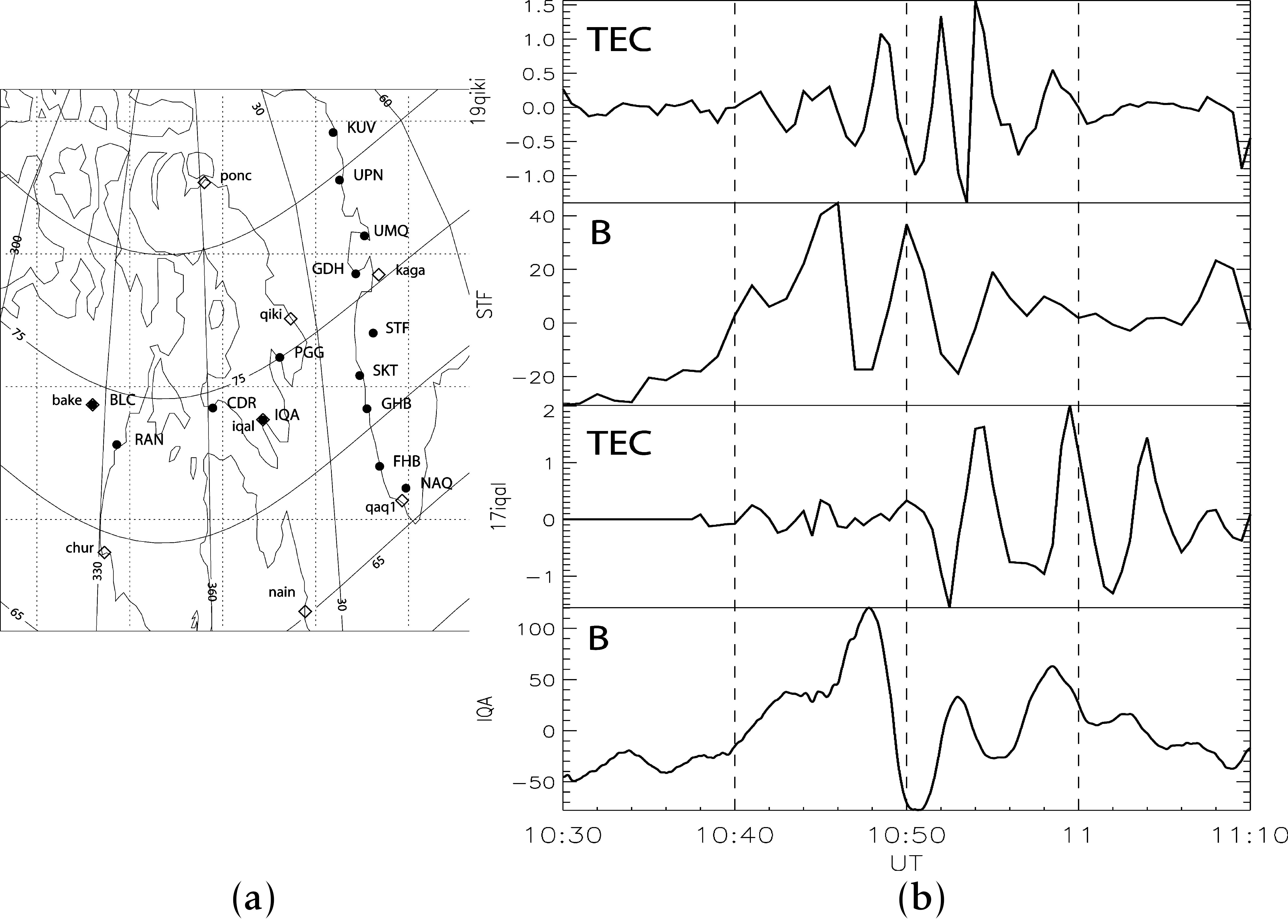
The use of array of GPS receivers and magnetometers in Arctic Canada and Greenland gave a possibility to monitor the origin and dynamics of isolated TCV-associated disturbance upon propagation along the ionosphere (Figure 12a) [Pronin et al., 2019]. This disturbance had a form of a TEC burst with rather high amplitude, ROT \(\geq 5\) TECu/min (Figure 12b). The field-aligned current system associated with the westward traveling TCV created TEC enhancement within a relatively narrow band of latitudes. The calculated horizontal propagation speed of the ionospheric disturbance was about a few km/s. Interestingly, the westward propagation speed estimated using the TEC observations was a factor of 2 slower than that using the ground magnetometer observations. These results prove that GNSS/TEC technique is sufficiently sensitive to monitor the formation and movement of TCV, though TEC response is not simply a “copy” of magnetic field disturbance.

3.8 Poloidal Small-Scale Alfvén Mode

Poloidal Pc4–5 pulsations are azimuthally small-scale (\(m \gg 1\)) Alfvén modes, generated by instabilities of energetic magnetospheric particles. Because of their small transverse scale, they are screened from ground magnetometers. A breakthrough in studies of such small-scale ULF waves, described as storm-time Pc5 pulsations or poloidal Alfvén modes, was achieved after the introduction of the ionospheric Scandinavian Twin Auroral Radar Experiment (STARE) radar [Walker et al., 1982]. Radar measurements gave a possibility to determine a 2D spatial structure (azimuthal wave number \(m\) and radial structure) of such small-scale Pc5 waves. Thus, poloidal Alfvén waves can be detected in the ionosphere by sensitive sounding techniques, such as radar [Bland et al., 2014; Ponomarenko et al., 2005] or Doppler sounder [Baddeley et al., 2005]. It is challenging to examine the possibility of using GNSS/TEC technique to detect small-scale ULF waves that are not observable with ground-based magnetometers. With the help of this technique, specific ULF modes generated upon the terminator movement along the ionosphere were revealed [Afraimovich et al., 2009].

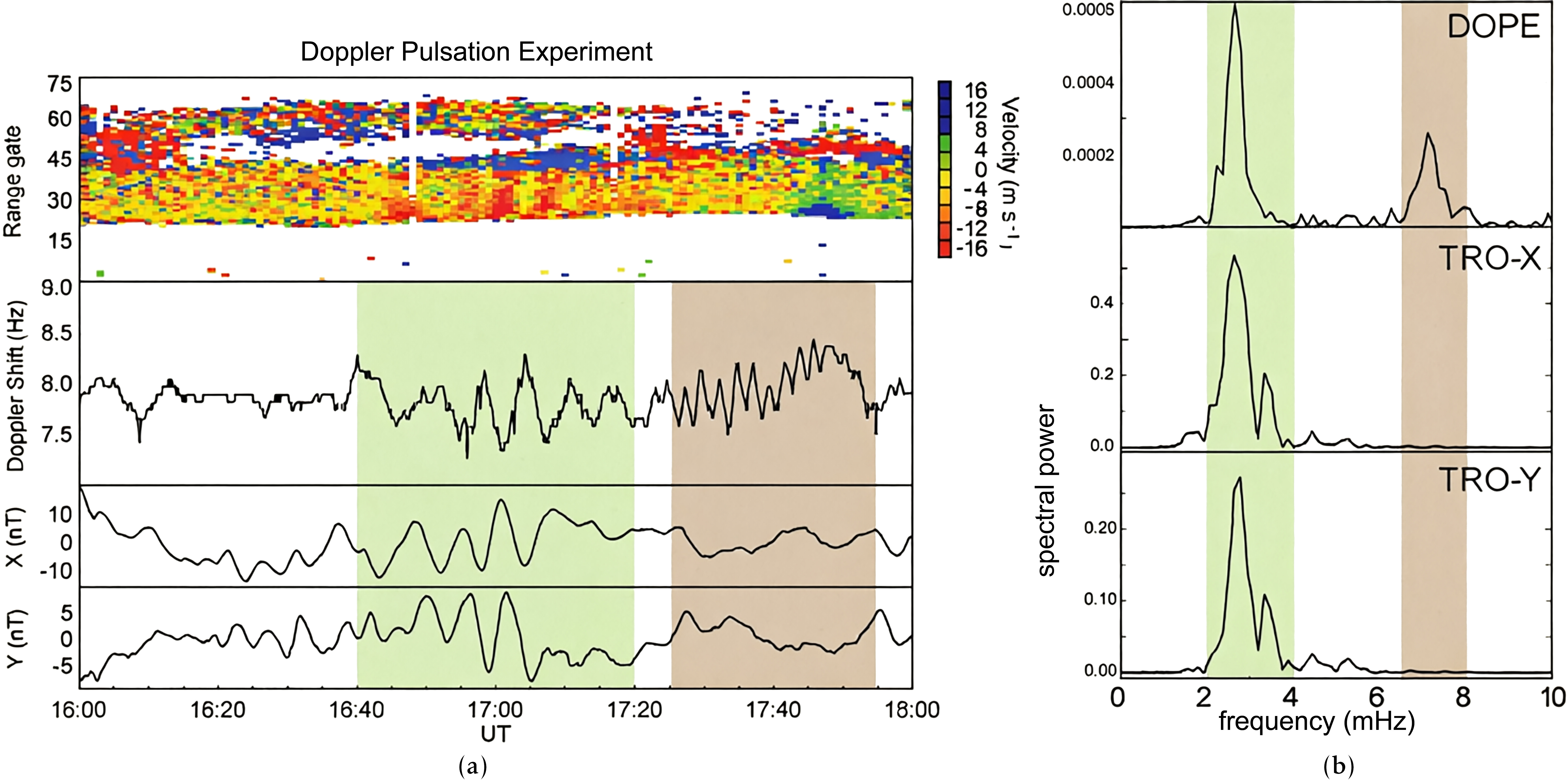
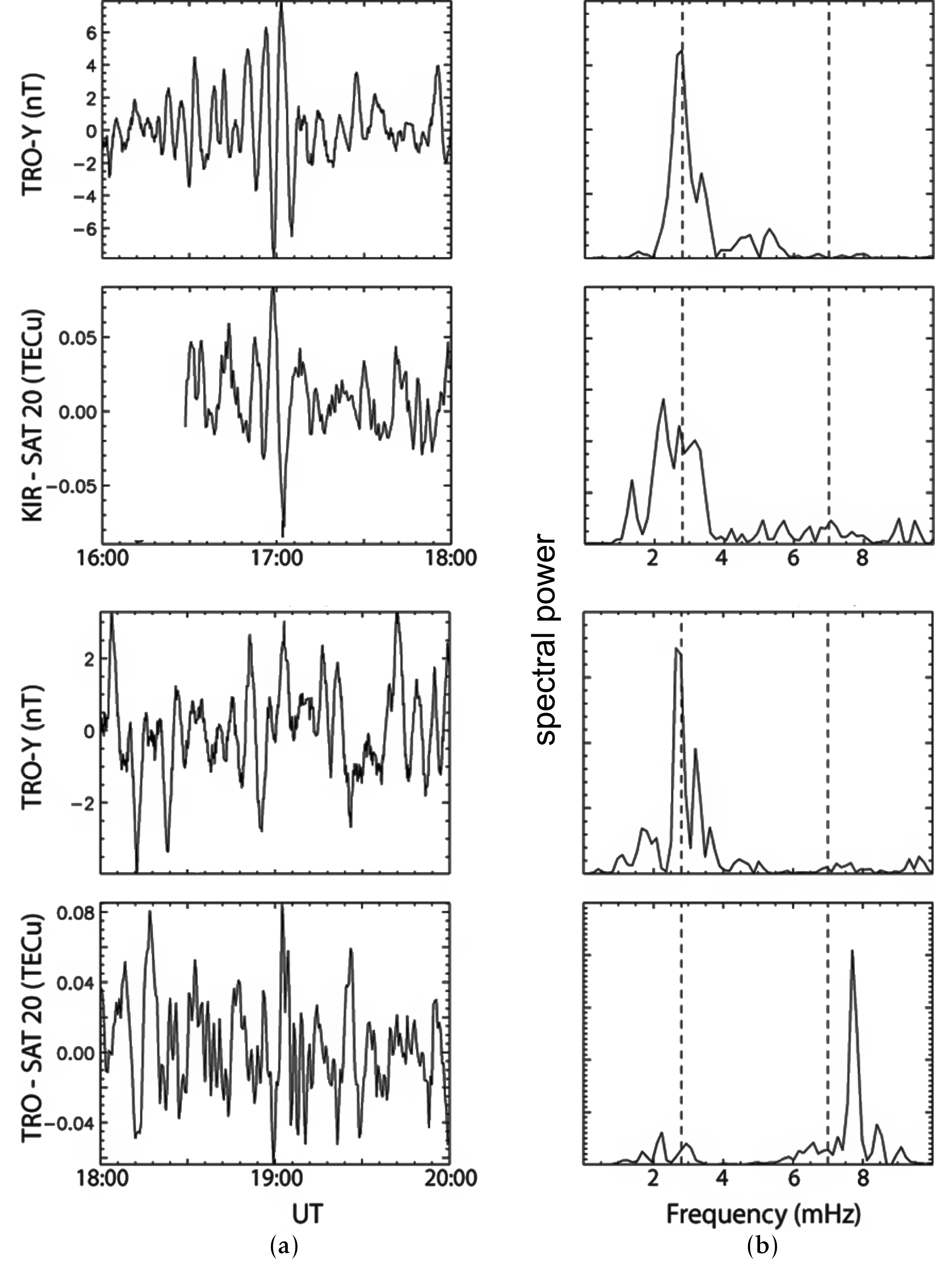
In the event recorded by Doppler sounder DOPE (Doppler Pulsation Experiment) both toroidal large-scale Pc5 pulsations and poloidal small-scale Pc4 pulsations were detected [Baddeley et al., 2005]. The large-scale Pc5 pulsations were evident in magnetometer and DOPE records (Figure 13). However, the small-scale poloidal Alfvén pulsations evident in DOPE spectra could not be seen by ground magnetometers. At the same time, Pc5 pulsations were observable in TEC data as well (Figure 14). Moreover, in TEC records fluctuations with period of poloidal Pc4 pulsation could be seen.

So far, the possibility of detecting small-scale ULF waves by the GNSS/TEC technique has only just started to be explored. Though poloidal waves are screened by the ionosphere from ground magnetometers, TEC data reliably captured signatures of these high-\(m\) waves similar to those seen in GOES data and SuperDARN velocity observations [Zhai et al., 2021]. Based on measurements from multiple GPS receivers 2D spatial structures of high-\(m\) ULF waves in the ionosphere can be revealed.

3.9 Possible Mechanisms of the Ionosphere Modulation by MHD Waves

Nearly 90% of TEC is provided by the ionospheric plasma at altitudes less than 10\(^3\) km. The temporal variations in the TEC evaluated along the radiopath between a source (S) and receiver (R), \(N_{\mathrm {T}}\), \[ N_{\mathrm {T}} = \int _{S}^{R} N \, \mathrm {d}s, \] where variations of local plasma density \(N\) are governed by the electron continuity equation \[ \frac {\partial N}{\partial t} = Q - L - \nabla \cdot (N \mathbf {V}). \]

Here \(Q\) and \(L\) are the electron production and loss rates respectively, \(\mathbf {V}\) is the plasma velocity produced by the ULF perturbation that may cause the density variations owing to plasma advection and divergence. Many possible mechanisms of periodic TEC modulation by incident MHD waves have been suggested:

1. Periodic ionization owing to the ULF-modulated precipitation of soft electrons into the ionosphere \(\propto Q(t)\) [Rodger et al., 2012]. Such electron fluxes should be absorbed predominantly in the F-layer to cause an observed TEC modulation. Periodic modulation of precipitating soft electrons by Alfvén wave may occur in the auroral acceleration region with field-aligned potential drop [Fedorov et al., 2004]. Precipitation of more energetic electrons absorbed in the bottom ionosphere detected by riometer observations hardly can produce noticeable effect on TEC;
2. Plasma compression by compressional-mode wave arising upon the interaction of an Alfvén wave with the anisotropic ionosphere \(\propto \nabla \mathbf {V}\) [Pilipenko et al., 2013]. This evanescent wave is excited by incident Alfvén waves owing to the E-layer Hall conductance. However, though the excitation rate increases for small-scale incident waves, a fast decay of an evanescent mode amplitude upward ~\(\exp (-kz)\) may suppresses the effect of TEC modulation;
3. Periodic advection across a lateral gradient of the ionospheric plasma [Waters and Cox, 2009]. However, the mechanism of plasma drift across a plasma gradient can be important only for very steep ionospheric inhomogeneities (e.g., polar cap patches);
4. Vertical shift and reconfiguration of the plasma vertical profile \(\partial N_{\mathrm {e}}/\partial z\) [Poole and Sutcliffe, 1987]. The finite East-West \(E_{y}\) component of an incident wave causes a vertical plasma drift \(V_{z} = E_{y}/B_{0} \sin I\), where \(I\) is the geomagnetic field inclination. Owing to the strong dependence of the ionization \(Q(z)\) and recombination \(L(z)\) rates on altitude \(z\), the vertical shift \(V_{z}\) causes a plasma modification due to the changes of ionization-recombination balance;
5. Frictional heating of ionospheric ions owing to periodic dragging by wave electric field through neutrals [Lathuillere et al., 1986]. This additional plasma heating may shift periodically the ionization-recombination balance due to the temperature-dependent recombination rate \(L(T)\) and cause plasma density variations.
6. Field-aligned plasma transport by Alfvén wave [Pilipenko et al., 2014b]. The field-aligned plasma and current transported by an Alfvén wave provides an additional periodic plasma flow into the bottom ionosphere and plasma density pumping/depleting in this region.

Too many proposed mechanisms mean that we still do not know the actual one. Therefore, the TEC modulation by Pc5 waves is a challenge for the MHD wave theory because the mechanism responsible for such modulation has not been firmly established yet.

4 Discussion

Our current knowledge of the ULF wave physics has been acquired mainly with the help of ground-based or satellite-borne magnetometers. However, their capabilities are limited, because even LEO satellites cannot detect in situ long-period ULF waves in the ionosphere — the region where energy flows from the magnetosphere into the upper atmosphere. Moreover, the ionosphere screens transversely small-scale structures (\(< 100\) km) from ground magnetometers. Ionospheric radars have emerged as a valuable source of additional information for ULF wave studies. GNSS/TEC observations are expected to provide new information about MHD wave interaction with the ionosphere. Modern multi-system GNSS receivers (even personal mobile phones) can simultaneously see 40–50 GNSS satellites of different systems. About 40 servers and data repositories in the world provide information on TEC derived from GNSS observations. Construction of global ionospheric maps (GIMs) is becoming a usual tool for the examination of 2D structure of ionospheric disturbances. Possibilities of conjunction studies with multiple types of instruments are expanding to understand the relevant physical process.

The radar community has demonstrated that Pc5/Pi3 waves can modulate the ionospheric electric field and plasma convection velocity, field-aligned current, electron density, the ionospheric conductance, electron and ion temperatures in both F and E layers. Recent observations summarized in this review have demonstrated that Pc5 waves are capable of modulating TEC as well. However, a possible mechanism of the modification of the ionosphere by magnetospheric ULF disturbance has not been established yet. Therefore, an examination of the impact on the ionosphere by disturbances of different physical nature, using simultaneous data from magnetometers and various ionospheric sounding techniques: (radars, riometers, and GNSS receivers), may provide an insight into the mechanism of the magnetosphere-ionosphere coupling.

So far, most work focused on single event studies. The first statistical study using THEMIS (Time History of Events and Macroscale Interactions during Substorms) satellite conjunctions with a ground-based magnetometer and GNSS receiver found that magnetospheric ULF waves generated TEC variations across the broad range of frequencies (\(\sim \)2–50 mHz), and that ULF TEC wave power was correlated with geomagnetic indices and magnetic field wave power in the magnetosphere and on the ground [Hartinger et al., 2025]. It was found that magnetospheric ULF waves can generate TEC variations with amplitudes up to ~4 TECu (\(\sim \)30% background) at local times near midnight.

Because of limited temporal resolution of most GNSS data (30 s) practically all ULF studies concentrated on disturbances in the Pc5-6 band. Nonetheless, there were reports indicating that Pc3 pulsations (periods of about a few tens seconds) can produce TEC fluctuations [Skone, 2009]. However, it is surprising how such small-amplitude geomagnetic pulsations (\(< 1\) nT) can induce TEC pulsations with amplitude ~0.1 TECu.

Why might the effects of the ionosphere modification by ULF waves be important for practical purposes? The ionospheric plasma modulation can influence the trans-ionospheric radio wave propagation [Sinha et al., 2002]. It can also impact space-borne technological systems like navigation and communication [Hernandez-Pajares et al., 2011]. Large ULF TEC variations may lead to scintillation through, for example, precipitation that leads to ionospheric irregularities [Kim et al., 2014; Shen et al., 2024; Tsunoda, 1988; Yizengaw et al., 2018]. More work is needed to determine the relationships between ULF TEC waves and the level of ionospheric scintillations.

In the same ULF frequency band, around 10 mins, the ionosphere is under regular impact from acoustic-gravity waves. Both acoustic-gravity waves and MHD waves provide a response in the geomagnetic field and in ionospheric parameters measured by radars and GNSS. How can one discriminate MHD wave impact from acoustic-gravity wave forcing? Probably, an effective impedance, similar to the impedance method used to discriminate contributions of Alfvén and compressional MHD modes [Pilipenko et al., 2012] can be introduced. For that, a theory of wave interaction with the ionosphere-atmosphere-ground system must predict the ratios between amplitudes of disturbances in ionospheric plasma velocity \(\mathbf {V}\), TEC \(\Delta N_{\mathrm {T}}\), and geomagnetic field \(\Delta B\), such as \(V/\Delta B\), \(\Delta N_{\mathrm {T}}/V\), \(\Delta N_{\mathrm {T}}/\Delta B\). Such relationships are a challenge for ULF theorists and modelers.

Remote sensing techniques for magnetospheric ULF wave fields are needed for many space weather applications, including quantifying radial transport rates in radiation belt and ring current models. The existing ground-based magnetometer and satellite measurements suffer from significant gaps in spatial coverage and, in the case of ground magnetometers, cannot detect certain ULF wave modes that are screened by the ionosphere. TEC obtained from GNSS receivers has been proposed as a complementary tool for remote sensing of magnetospheric ULF wave properties. Moreover, the addition of GNSS receivers would improve spatial coverage of ULF wave observations and potential for coverage over oceans via buoy networks. So far, no studies have established a statistical connection between ULF wave amplitudes observed in geomagnetic field and TEC, which is needed to use TEC as a proxy for ULF amplitude. There is some doubt whether such a simple connection exists, given the range of potential mechanisms driving ULF TEC.

All ULF wave models assume a static ionosphere with at most small linear disturbances in ionospheric parameters related to the waves. A case study using radar measurements [Wang et al., 2020] discovered large variations (up to 60%) in ionospheric parameters, inconsistent with predictions from linear theory. Therefore, sometimes linear theory may not be adequate to describe these large disturbances, with implications for wave reflection coefficients and overall dynamics, ionosphere-thermosphere heating rates and wave dissipation rates. For such events the magnetospheric field line resonator cannot be imagined as an Alfvén resonator terminated by two steady ionospheric reflective “mirrors”.

5 Conclusion

Long-period geomagnetic Pc5 pulsations, being the most powerful wave process in the terrestrial environment, can significantly modulate the local densities of the magnetospheric and ionospheric plasma. Even radio-path-integrated TEC has turned out to be sensitive enough to respond to various types of long-period ULF waves and transients. GNSS/TEC technique can be effectively used as an additional tool for the study of ULF wave physics in the near-Earth space. So far, the effect of TEC modulation by ULF waves is a challenge for the MHD wave theory, because mechanisms responsible for such modulation have not been firmly established yet.

Acknowledgments. The study is supported by the grant No. 24-77-10012 from the Russian Science Foundation.

1. Afraimovich, E. L., E. I. Astafyeva, V. V. Demyanov, et al. 2013. “A review of GPS/GLONASS studies of the ionospheric response to natural and anthropogenic processes and phenomena.” Journal of Space Weather and Space Climate 3: A27. https://doi.org/10.1051/swsc/2013049

2. Afraimovich, E. L., I. K. Edemskiy, A. S. Leonovich, L. A. Leonovich, S. V. Voeykov, and Y. V. Yasyukevich. 2009. “MHD nature of night-time MSTIDs excited by the solar terminator.” Geophysical Research Letters 36 (15): L15106. https://doi.org/10.1029/2009gl039803

3. Alfonsi, L., N. Bergeot, P. Cilliers, et al. 2022. “Review of environmental monitoring by means of radio waves in the polar regions: From atmosphere to geospace.” Surveys in Geophysics 43 (6): 1609–98. https://doi.org/10.1007/s10712-022-09734-z

4. Astafyeva, E. 2019. “Ionospheric detection of natural hazards.” Reviews of Geophysics 57 (4): 1265–88. https://doi.org/10.1029/2019RG000668

5. Astafyeva, E., and K. Shults. 2019. “Ionospheric GNSS imagery of seismic source: Possibilities, difficulties, and challenges.” Journal of Geophysical Research: Space Physics 124 (1): 534–43. https://doi.org/10.1029/2018JA026107

6. Baddeley, L. J., T. K. Yeoman, and D. M. Wright. 2005. “HF doppler sounder measurements of the ionospheric signatures of small scale ULF waves.” Annales Geophysicae 23 (5): 1807–20. https://doi.org/10.5194/angeo-23-1807-2005

7. Belakhovsky, V. B., V. A. Pilipenko, Ya. A. Sakharov, et al. 2017. “Geomagnetic and ionospheric response to the interplanetary shock on January 24, 2012.” Earth, Planets and Space 69 (1): 105. https://doi.org/10.1186/s40623-017-0696-1

8. Belakhovsky, V. B., V. A. Pilipenko, and S. N. Samsonov. 2017. “The simultaneous ULF waves in geomagnetic field, TEC of the ionosphere, aurora intensity and cosmic noise absorption.” Transactions of the Kola Science Centre of the RAS 8 (7–3): 55–60

9. Belakhovsky, V., V. Pilipenko, D. Murr, et al. 2016. “Modulation of the ionosphere by Pc5 waves observed simultaneously by GPS/TEC and EISCAT.” Earth, Planets and Space 68 (1). https://doi.org/10.1186/s40623-016-0480-7

10. Bland, E. C., and A. J. McDonald. 2016. “High spatial resolution radar observations of ultralow frequency waves in the southern polar cap.” Journal of Geophysical Research: Space Physics 121 (5): 4005–16. https://doi.org/10.1002/2015ja022235

11. Bland, E. C., A. J. McDonald, F. W. Menk, and J. C. Devlin. 2014. “Multipoint visualization of ULF oscillations using the Super Dual Auroral Radar Network.” Geophysical Research Letters 41 (18): 6314–20. https://doi.org/10.1002/2014gl061371

12. Buchert, S. C., R. Fujii, and K.-H. Glassmeier. 1999. “Ionospheric conductivity modulation in ULF pulsations.” Journal of Geophysical Research: Space Physics 104 (A5): 10119–33. https://doi.org/10.1029/1998JA900180

13. Crowley, G., N. Wade, J. A. Waldock, et al. 1985. “High time-resolution observations of periodic frictional heating associated with a Pc5 micropulsation.” Nature 316 (6028): 528–30. https://doi.org/10.1038/316528a0

14. Davies, K., and G. K. Hartmann. 1976. “Short-period fluctuations in total columnar electron content.” Journal of Geophysical Research 81 (19): 3431–34. https://doi.org/10.1029/ja081i019p03431

15. Fedorov, E., V. Pilipenko, M. J. Engebretson, and T. J. Rosenberg. 2004. “Alfven wave modulation of the auroral acceleration region.” Earth, Planets and Space 56 (7): 649–61. https://doi.org/10.1186/bf03352527

16. Fenrich, F. R., C. L. Waters, M. Connors, and C. Bredeson. 2006. “Ionospheric signatures of ULF waves: Passive radar techniques.” In Magnetospheric ULF Waves: Synthesis and New Directions. American Geophysical Union. https://doi.org/10.1029/169gm17

17. Galvan, D. A., A. Komjathy, M. P. Hickey, and A. J. Mannucci. 2011. “The 2009 Samoa and 2010 Chile tsunamis as observed in the ionosphere using GPS total electron content.” Journal of Geophysical Research: Space Physics 116 (A6). https://doi.org/10.1029/2010ja016204

18. Gjerloev, J. W., R. A. Greenwald, C. L. Waters, et al. 2007. “Observations of Pi2 pulsations by the Wallops HF radar in association with substorm expansion.” Geophysical Research Letters 34 (20). https://doi.org/10.1029/2007gl030492

19. Hartinger, M. D., X. Shi, O. Verkhoglyadova, et al. 2025. “Statistical analysis of ultra-low-frequency total electron content disturbances: Relationship to magnetospheric waves.” Journal of Geophysical Research: Space Physics 130 (4): e2024JA033456. https://doi.org/10.1029/2024JA033456

20. Hazendonk, C. M. van, L. Baddeley, K. M. Laundal, and J. L. Chau. 2024. “Detection and energy dissipation of ULF waves in the polar ionosphere: A case study using the EISCAT radar.” Journal of Geophysical Research: Space Physics 129 (7). https://doi.org/10.1029/2024JA032633

21. Hernandez-Pajares, M., J. M. Juan, J. Sanz, et al. 2011. “The ionosphere: effects, GPS modeling and the benefits for space geodetic techniques.” Journal of Geodesy 85 (12): 887–907. https://doi.org/10.1007/s00190-011-0508-5

22. Huang, C. Y., J. F. Helmboldt, J. Park, et al. 2019. “Ionospheric detection of explosive events.” Reviews of Geophysics 57 (1): 78–105. https://doi.org/10.1029/2017RG000594

23. Kim, H., C. R. Clauer, K. Deshpande, et al. 2014. “Ionospheric irregularities during a substorm event: Observations of ULF pulsations and GPS scintillations.” Journal of Atmospheric and Solar-Terrestrial Physics 114: 1–8. https://doi.org/10.1016/j.jastp.2014.03.006

24. Kivelson, M. G., and D. J. Southwood. 1991. “Ionospheric traveling vortex generation by solar wind buffeting of the magnetosphere.” Journal of Geophysical Research: Space Physics 96 (A2): 1661–67. https://doi.org/10.1029/90ja01805

25. Komjathy, A., D. A. Galvan, P. Stephens, et al. 2012. “Detecting ionospheric TEC perturbations caused by natural hazards using a global network of GPS receivers: The Tohoku case study.” Earth, Planets and Space 64 (12): 1287–94. https://doi.org/10.5047/eps.2012.08.003

26. Kozyreva, O. V., V. A. Pilipenko, E. C. Bland, et al. 2020. “Periodic Modulation of the Upper Ionosphere by ULF Waves as Observed Simultaneously by SuperDARN Radars and GPS/TEC Technique.” Journal of Geophysical Research: Space Physics 125 (7): e2020JA028032. https://doi.org/10.1029/2020ja028032

27. Lanzerotti, L. J., R. D. Hunsucker, D. Rice, et al. 1987. “Ionosphere and ground-based response to field-aligned currents near the magnetospheric cusp regions.” Journal of Geophysical Research: Space Physics 92 (A7): 7739–43. https://doi.org/10.1029/ja092ia07p07739

28. Lathuillere, C., F. Glangeaud, and Z. Y. Zhao. 1986. “Ionospheric ion heating by ULF Pc 5 magnetic pulsations.” Journal of Geophysical Research: Space Physics 91 (A2): 1619–26. https://doi.org/10.1029/ja091ia02p01619

29. Lester, M., J. A. Davies, and T. K. Yeoman. 2000. “Letter to the editor: The ionospheric response during an interval of Pc5 ULF wave activity.” Annales Geophysicae 18 (2): 257–61. https://doi.org/10.1007/s00585-000-0257-x

30. Lin, D., M. Hartinger, W. Lotko, et al. 2025. “Efficiency of Electromagnetic Energy Transfer From Solar Wind to Ionosphere Through Magnetospheric Ultra-Low Frequency Waves.” Geophysical Research Letters 53 (1): e2025GL118532. https://doi.org/10.1029/2025gl118532

31. Marin, J., V. Pilipenko, O. Kozyreva, et al. 2014. “Global Pc5 pulsations during strong magnetic storms: excitation mechanisms and equatorward expansion.” Annales Geophysicae 32 (4): 319–31. https://doi.org/10.5194/angeo-32-319-2014

32. McHenry, M. A., and C. R. Clauer. 1987. “Modeled ground magnetic signatures of flux transfer events.” Journal of Geophysical Research: Space Physics 92 (A10): 11231–40. https://doi.org/10.1029/ja092ia10p11231

33. Meng, X., P. Vergados, A. Komjathy, and O. Verkhoglyadova. 2019. “Upper atmospheric responses to surface disturbances: an observational perspective.” Radio Science 54 (11): 1076–98. https://doi.org/10.1029/2019rs006858

34. Menk, F. W., C. L. Waters, and S. I. Dunlop. 2007. “ULF Doppler oscillations in the low latitude ionosphere.” Geophysical Research Letters 34 (10). https://doi.org/10.1029/2007gl029300

35. Norouzi-Sedeh, L., C. L. Waters, and F. W. Menk. 2015. “Survey of ULF wave signatures seen in the Tasman International Geospace Environment Radars data.” Journal of Geophysical Research: Space Physics 120 (2): 949–63. https://doi.org/10.1002/2014JA020652

36. Okuzawa, T., and K. Davies. 1981. “Pulsations in total columnar electron content.” Journal of Geophysical Research: Space Physics 86 (A3): 1355–63. https://doi.org/10.1029/ja086ia03p01355

37. Pilipenko, V. A., M. Bravo, N. V. Romanova, et al. 2018. “Geomagnetic and ionospheric responses to the interplanetary shock wave of March 17, 2015.” Izvestiya, Physics of the Solid Earth 54 (5): 721–40. https://doi.org/10.1134/S1069351318050129

38. Pilipenko, V. A., E. N. Fedorov, M. Teramoto, and K. Yumoto. 2013. “The mechanism of mid-latitude Pi2 waves in the upper ionosphere as revealed by combined Doppler and magnetometer observations.” Annales Geophysicae 31 (4): 689–95. https://doi.org/10.5194/angeo-31-689-2013

39. Pilipenko, V., V. Belakhovsky, A. Kozlovsky, et al. 2012. “Determination of the wave mode contribution into the ULF pulsations from combined radar and magnetometer data: Method of apparent impedance.” Journal of Atmospheric and Solar-Terrestrial Physics 77: 85–95. https://doi.org/10.1016/j.jastp.2011.11.013

40. Pilipenko, V., V. Belakhovsky, A. Kozlovsky, et al. 2014. “ULF wave modulation of the ionospheric parameters: Radar and magnetometer observations.” Journal of Atmospheric and Solar-Terrestrial Physics 108: 68–76. https://doi.org/10.1016/j.jastp.2013.12.015

41. Pilipenko, V., V. Belakhovsky, D. Murr, et al. 2014. “Modulation of total electron content by ULF Pc5 waves.” Journal of Geophysical Research: Space Physics 119 (6): 4358–69. https://doi.org/10.1002/2013JA019594

42. Ponomarenko, P. V., F. W. Menk, C. L. Waters, and M. D. Sciffer. 2005. “Pc3-4 ULF waves observed by the SuperDARN TIGER radar.” Annales Geophysicae 23 (4): 1271–80. https://doi.org/10.5194/angeo-23-1271-2005

43. Ponomarenko, P. V., C. L. Waters, M. D. Sciffer, et al. 2001. “Spatial structure of ULF waves: Comparison of magnetometer and Super Dual Auroral Radar Network data.” Journal of Geophysical Research: Space Physics 106 (A6): 10509–17. https://doi.org/10.1029/2000ja000281

44. Poole, A. W. V., and P. R. Sutcliffe. 1987. “Mechanisms for observed total electron content pulsations at mid latitudes.” Journal of Atmospheric and Terrestrial Physics 49 (3): 231–36. https://doi.org/10.1016/0021-9169(87)90058-4

45. Potapov, A. S., E. Amata, T. N. Polyushkina, et al. 2011. “A case study of global ULF pulsations using data from space-borne and ground-based magnetometers and a SuperDARN radar.” Kosmíčna Nauka í Tehnologíâ 17 (6): 54–67. https://doi.org/10.15407/knit2011.06.054

46. Pronin, V. E., V. A. Pilipenko, V. I. Zakharov, et al. 2019. “Response of Ionospheric Total Electron Content to Convective Vortices.” Cosmic Research 57 (2): 69–78. https://doi.org/10.1134/s0010952519020072

47. Rodger, C. J., M. A. Clilverd, A. J. Kavanagh, et al. 2012. “Contrasting the responses of three different ground-based instruments to energetic electron precipitation.” Radio Science 47 (2): RS2021. https://doi.org/10.1029/2011RS004971

48. Sakaguchi, K., T. Nagatsuma, T. Ogawa, T. Obara, and O. A. Troshichev. 2012. “Ionospheric Pc5 plasma oscillations observed by the King Salmon HF radar and their comparison with geomagnetic pulsations on the ground and in geostationary orbit.” Journal of Geophysical Research: Space Physics 117 (A3). https://doi.org/10.1029/2011ja016923

49. Shalimov, S. L., A. A. Rozhnoi, M. S. Solov’eva, and E. V. Ol’shanskaya. 2019. “Impact of earthquakes and tsunamis on the ionosphere.” Izvestiya, Physics of the Solid Earth 55 (1): 168–81. https://doi.org/10.1134/s1069351319010087

50. Shen, Y., O. P. Verkhoglyadova, A. Artemyev, et al. 2024. “Magnetospheric control of ionospheric TEC perturbations via whistler-mode and ULF waves.” AGU Advances 5 (6): e2024AV001302. https://doi.org/10.1029/2024AV001302

51. Shi, X., J. M. Ruohoniemi, J. B. H. Baker, et al. 2018. “Survey of Ionospheric Pc3-5 ULF Wave Signatures in SuperDARN High Time Resolution Data.” Journal of Geophysical Research: Space Physics 123 (5): 4215–31. https://doi.org/10.1029/2017JA025033

52. Shinbori, A., K. Hosokawa, T. Hori, et al. 2024. “Periodic oscillations in the high-latitude ionosphere driven by ultralow frequency waves: simultaneous measurements using SuperDARN radars and GNSS-TEC technique.” Preprint. Research Square, ahead of print. https://doi.org/10.21203/rs.3.rs-4001720/v1

53. Sinha, A. K., B. M. Pathan, R. Rajaram, and D. R. K. Rao. 2002. “Low frequency modulation of transionospheric radio wave amplitude at low-latitudes: possible role of field line oscillations.” Annales Geophysicae 20 (1): 69–80. https://doi.org/10.5194/angeo-20-69-2002

54. Skone, S. 2009. “Using GPS TEC measurements to detect geomagnetic Pc 3 pulsations.” Radio Science 44 (1): RS0A27. https://doi.org/10.1029/2008rs004106

55. Teramoto, M., N. Nishitani, V. Pilipenko, et al. 2014. “Pi2 pulsation simultaneously observed in the E and F region ionosphere with the SuperDARN Hokkaido radar.” Journal of Geophysical Research: Space Physics 119 (5): 3444–62. https://doi.org/10.1002/2012JA018585

56. Tsai, H.-F., J.-Y. Liu, C.-H. Lin, and C.-H. Chen. 2011. “Tracking the epicenter and the tsunami origin with GPS ionosphere observation.” Earth, Planets and Space 63 (7): 859–62. https://doi.org/10.5047/eps.2011.06.024

57. Tsunoda, R. T. 1988. “High-latitude F region irregularities: A review and synthesis.” Reviews of Geophysics 26 (4): 719–60. https://doi.org/10.1029/rg026i004p00719

58. Vesnin, A., Y. Yasyukevich, N. Perevalova, and E. Şentürk. 2023. “Ionospheric response to the 6 February 2023 Turkey-Syria earthquake.” Remote Sensing 15 (9): 2336. https://doi.org/10.3390/rs15092336

59. Vorontsova, E., V. Pilipenko, E. Fedorov, et al. 2016. “Modulation of total electron content by global Pc5 waves at low latitudes.” Advances in Space Research 57 (1): 309–19. https://doi.org/10.1016/j.asr.2015.10.041

60. Walker, A. D. M., R. A. Greenwald, A. Korth, and G. Kremser. 1982. “STARE and GEOS 2 observations of a storm time Pc 5 ULF pulsation.” Journal of Geophysical Research: Space Physics 87 (A11): 9135–46. https://doi.org/10.1029/ja087ia11p09135

61. Wang, B., Y. Nishimura, M. Hartinger, et al. 2020. “Ionospheric Modulation by Storm Time Pc5 ULF Pulsations and the Structure Detected by PFISR-THEMIS Conjunction.” Geophysical Research Letters 47 (16): e2020GL089060. https://doi.org/10.1029/2020gl089060

62. Waters, C. L., and S. P. Cox. 2009. “ULF wave effects on high frequency signal propagation through the ionosphere.” Annales Geophysicae 27 (7): 2779–88. https://doi.org/10.5194/angeo-27-2779-2009

63. Waters, C. L., T. K. Yeoman, M. D. Sciffer, et al. 2007. “Modulation of radio frequency signals by ULF waves.” Annales Geophysicae 25 (5): 1113–24. https://doi.org/10.5194/angeo-25-1113-2007

64. Watson, C., P. T. Jayachandran, H. J. Singer, et al. 2015. “Large-amplitude GPS TEC variations associated with Pc5-6 magnetic field variations observed on the ground and at geosynchronous orbit.” Journal of Geophysical Research: Space Physics 120 (9): 7798–821. https://doi.org/10.1002/2015ja021517

65. Watson, C., P. T. Jayachandran, H. J. Singer, et al. 2016. “GPS TEC response to Pc4 "giant pulsations".” Journal of Geophysical Research: Space Physics 121 (2): 1722–35. https://doi.org/10.1002/2015JA022253

66. Wright, D. M., T. K. Yeoman, and J. A. Davies. 1998. “A comparison of EISCAT and HF Doppler observations of a ULF wave.” Annales Geophysicae 16 (10): 1190–99. https://doi.org/10.1007/s00585-998-1190-7

67. Yasyukevich, Y. V., A. M. Vesnin, E. Astafyeva, B. M. Maletckii, V. P. Lebedev, and A. M. Padokhin. 2024. “Supersonic waves generated by the 18 November 2023 Starship flight and explosions: Unexpected northward propagation and a man-made non-chemical depletion.” Geophysical Research Letters 51 (16). https://doi.org/10.1029/2024GL109284

68. Yizengaw, E., E. Zesta, M. B. Moldwin, et al. 2018. “ULF Wave-Associated Density Irregularities and Scintillation at the Equator.” Geophysical Research Letters 45 (11): 5290–98. https://doi.org/10.1029/2018gl078163

69. Zhai, C., X. Shi, W. Wang, et al. 2021. “Characterization of High-m ULF Wave Signatures in GPS TEC Data.” Geophysical Research Letters 48 (14): e2021GL094282. https://doi.org/10.1029/2021gl094282

70. Ziesolleck, C. W. S., F. R. Fenrich, J. C. Samson, and D. R. McDiarmid. 1998. “Pc5 field line resonance frequencies and structure observed by SuperDARN and CANOPUS.” Journal of Geophysical Research: Space Physics 103 (A6): 11771–85. https://doi.org/10.1029/98ja00590