












Moscow, Russian Federation
UDC 55
UDC 550.34
UDC 550.383
CSCSTI 37.01
CSCSTI 37.15
CSCSTI 37.25
CSCSTI 37.31
CSCSTI 38.01
CSCSTI 36.00
CSCSTI 37.00
CSCSTI 38.00
CSCSTI 39.00
CSCSTI 52.00
Russian Classification of Professions by Education 05.00.00
Russian Library and Bibliographic Classification 26
Russian Trade and Bibliographic Classification 63
BISAC SCI SCIENCE
In the subduction zone of the Kamchatka Peninsula, where the powerful earthquake (Mw 8.2–8.8) of July 29, 2025, repeated the hypocenter location of the 1952 event, the task of studying the spatial heterogeneity of interseismic deformation as an indicator of the preparation for major seismic events is relevant. The aim of this work was to identify large geodynamic blocks with similar deformation parameters in the southern part of Kamchatka based on data analysis for the period preceding the specified seismic activity. A methodology that combines radar interferometry (the SBAS method implemented in the MintPy package) and Global Navigation Satellite System (GNSS) data was applied and adapted for this purpose. The technique was specifically developed for the conditions of Kamchatka – Russia's snowiest region with high atmospheric turbulence. It includes using data exclusively from the snow-free period (May–October) with a coherence threshold of 0.75; integrating GNSS measurements to fill gaps in the SBAS time series and build continuous velocity fields; and correcting for atmospheric delays. As a result of processing Sentinel-1 data for 2017–2025 and clustering the velocity fields by two components (vertical and west–east direction), a clear division of the territory into two large blocks – western and eastern – separated by a buffer zone, was revealed. It was established that the displacement rate of the eastern block (19.3–21.0 mm/yr) is several times higher than that of the western block (4.6–8.7 mm/yr). The obtained results demonstrate the effectiveness of the proposed synergistic approach for mapping the block structure and quantifying interseismic deformations in complex natural conditions, which is important for assessing seismic hazard in subduction zones.
Geodynamics, interseismic deformation, lithospheric block structure, radar interferometry, deformation mapping, July 29, 2025 earthquake, subduction zone, kamchatka megathrust earthquake
1 Introduction
The Kamchatka Peninsula is one of the most seismically active regions in the world, where key tectonic structures of the northwestern Pacific Ring of Fire (also known as the Circum-Pacific Belt) intersect. Monitoring its geodynamics is fundamental for understanding the cyclicity of major earthquakes.
A series of powerful seismic events occurred off the eastern coast of Kamchatka on July 29, 2025. According to data from the USGS Earthquake Hazards Program (https://earthquake.usgs.gov), the European-Mediterranean Seismological Centre (https://www.emsc-csem.org), and the Geophysical Survey of Russia Academy of Sciences (http://www.ceme.gsras.ru/new/ssd_news.htm), the magnitude of the main shock ranged from \(Mw\) 8.2 to \(Mw\) 8.8 (coordinates: 52.43\(^\circ \)N, 160.46\(^\circ \)E, depth ~20 km) and was accompanied by numerous aftershocks with magnitudes up to \(Mw\) 7.8. Currently, a rupture surface model has been obtained that reliably describes coseismic displacements [Mikhailov et al., 2025]. Significantly, the hypocenter of this event almost completely coincides with the hypocenter of the Great Kamchatka Earthquake of 1952 (\(Mw=9.0\)). This indicates a high degree of spatial localization of the zones of maximum seismic moment and emphasizes the importance of studying interseismic deformation during intercycle periods lasting several decades for assessing the seismic hazard potential. Such estimates of interseismic displacements will be an important supplement to future studies of the region’s geodynamics and will also allow us to identify possible catalysts of seismic activity in addition to the process of plate subduction in this case, as was previously shown by the authors using the example of earthquakes in Morocco and Turkey [Bondur et al., 2024, 2025].
Key tools for quantitative assessment of slow tectonic deformations today include satellite geodesy methods, particularly differential radar interferometry (DInSAR), and global navigation satellite systems (GNSS). A synergistic approach is often used, where GNSS provides absolute accuracy and InSAR provides spatial interpolation, for example, in [Chen et al., 2025; Guo et al., 2023; Li et al., 2022; Tao et al., 2025]. It should be noted that the latter study used nine GNSS stations over a small area, while other studies used data from more than 20 GNSS stations. In turn, in the southern part of Kamchatka under study, there are only two stations. Nevertheless, the results of these studies suggest that each station qualitatively and, to some extent, quantitatively characterizes the geodynamics of its block. This raises the problem of spatially classifying territories into blocks with similar dynamics.
To analyze vast, sparsely developed areas in order to identify block structures, methods using long-term interferometric data series are most suitable. However, their application in Kamchatka, the snowiest region of Russia with a snow cover depth of 40 to 250 cm [Tananaev et al., 2025], is complicated by the strong influence of snow on signal coherence [Dagurov et al., 2020; Zakharov and Zakharova, 2023]. The PS-InSAR method [Ferretti et al., 2001], effective in areas with stable point scatterers, yields a sparse spatial structure in natural landscapes [Bondur et al., 2021]. The Stacking-InSAR (weighted averaging of interferograms) method [Zhang et al., 2021] was tested for assessing this earthquake in [Chimitdorzhiev et al., 2025]. However, it showed unsatisfactory results due to the complex natural and climatic conditions, primarily atmospheric inhomogeneities, even with the corrections applied (e.g., Generic Atmospheric Correction Online Service for InSAR – GACOS, http://www.gacos.net). This limits its application to areas with stable atmospheric conditions [Bondur et al., 2024, 2025] and makes it unsuitable for Kamchatka with its complex meteorology. Also, regarding atmospheric corrections in this region, it is necessary to point out a recent work [Volkova et al., 2025], which does not recommend “using default corrections without comparing the original and corrected displacement fields, but focusing on displacements that appeared after the corrections were applied.” In this context, the most promising approach is the Small BAseline Subset (SBAS) method [Berardino et al., 2002], which, by processing a large number of interferometric pairs with small temporal and spatial baselines, enables the retrieval of displacement fields for large areas while minimizing decorrelation effects, as well as for smaller areas with varying displacement dynamics [Tao et al., 2025].
Thus, the study aims to identify large block structures in Kamchatka with similar interseismic deformation parameters and assess their dynamics. To this end, the SBAS method is used to process multi-year interferometric data time series. The expected result is a map of the spatial distribution of displacement fields before the strongest seismic events.
2 Geoblock Classification: Methodology and Results
The research methodology implies the following conditions, limitations, and assumptions:
- Here we propose to estimate the deformation dynamics based on the processing of large volumes of C-band (wavelength 5.6 cm) Sentinel-1 radar interferometric data from 2017 until the date of the last survey before the seismic activity on July 29, 2025. In general, Sentinel-1 A/B radars have been surveying since 2014, but since 2017, the division of successive radar frames of one orbit has been carried out with a shift relative to the previous location. Therefore, in order to cover the maximum possible territory with a single frame, a time series since 2017 was selected;
- Kamchatka is characterized by a fairly thick, and in some years anomalous, snow cover, with depths varying from 40 to 250 cm in different parts of the peninsula [Tananaev et al., 2025]. This causes a serious problem for interferometric measurements: seasonal accumulation and melting of snow, especially with such different depths, leads to strong signal decorrelation and significant phase shifts, which reduces the reliability of the data [Dagurov et al., 2020; Zakharov and Zakharova, 2023]. To solve this problem, we propose to use data obtained from the second third of May to the end of October, i.e., during a period when a significant portion of the territory is completely free of snow or its presence is minimal. This will eliminate the majority of interferograms affected by snow cover. Additionally, when processing using the SBAS method, a coherence threshold of 0.75 will be applied to exclude pixels with low measurement reliability from consideration (for example, where the influence of snow in high-mountain regions or in transition months – May, September, and October – is possible), thereby increasing the overall accuracy of the resulting time series of displacements.
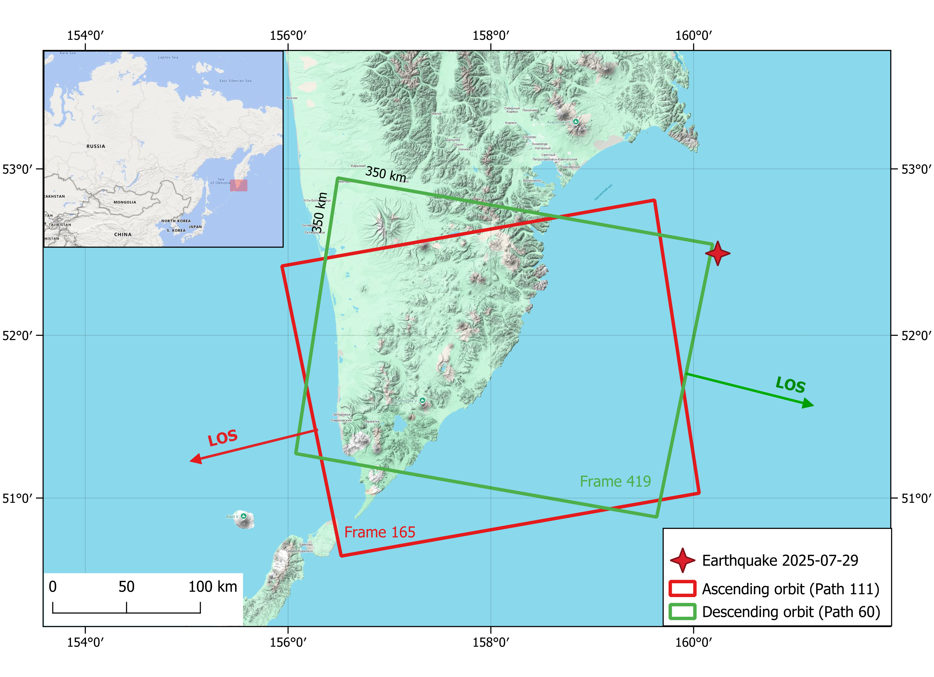
- The online platform Alaska Satellite Facility/span>s Hybrid Pluggable Processing Pipeline (ASF HyP3) [Hogenson et al., 2025] was used to obtain and process long-term series of radar interferometric data with its state-of-the-art functionality. This online platform provides access to Sentinel-1 radar data and allows data selection and interferometric processing, starting from image matching to obtaining the unwrapped phase. Time series of the latter with a spatial resolution of 80 m were used for the calculations. The outlines of the radar images on the ascending (321 images) and descending (275 images) orbits are presented in 1a. The arrows indicate the directions of positive displacements along the radar line of sight (LOS).
To derive the displacement velocity field, the open-source software package MinPy [Yunjun et al., 2019] was used. This package implements an advanced SBAS InSAR technique. MintPy offers a more automated, accurate, and flexible approach compared to classical SBAS, especially in challenging conditions (low coherence, deconvolution errors, nonlinear deformations). In MintPy, atmospheric (tropospheric) delay correction is performed in two main ways. Both methods are applied not at the interferogram level but in the time-series domain after inversion of the interferogram network.
The first main method is the use of global atmospheric models (GAMs), such as ERA-5, ERA-Interim, NARR, or MERRA. These models provide absolute tropospheric delay data for each pixel at each survey time, which is then converted into a relative delay between a given pixel and a reference pixel and subtracted from the phase time series. This approach is effective for correcting the stratified component of the delay, but its accuracy is limited by the spatiotemporal resolution of the models and may not adequately account for local turbulent components, especially in regions with complex topography, such as Kamchatka.
The second method is empirical correction, based on the linear dependence of delay on altitude. This can be effective in mountainous regions but has a drawback: it doesn/span>t distinguish between stratified tropospheric delay and real land surface displacements, which can also be correlated with topography (e.g., volcanic deformation), potentially removing informative signal phases.
Correction in MintPy is performed in stages: first, the tropospheric component estimated by one of these methods is subtracted, and then other components, such as topography, are corrected. Although the GAMs approach is the standard, its effectiveness for high-precision measurements in regions with intense summer convection and significant precipitation variations can be insufficient, and residual atmospheric noise often requires additional filtering.
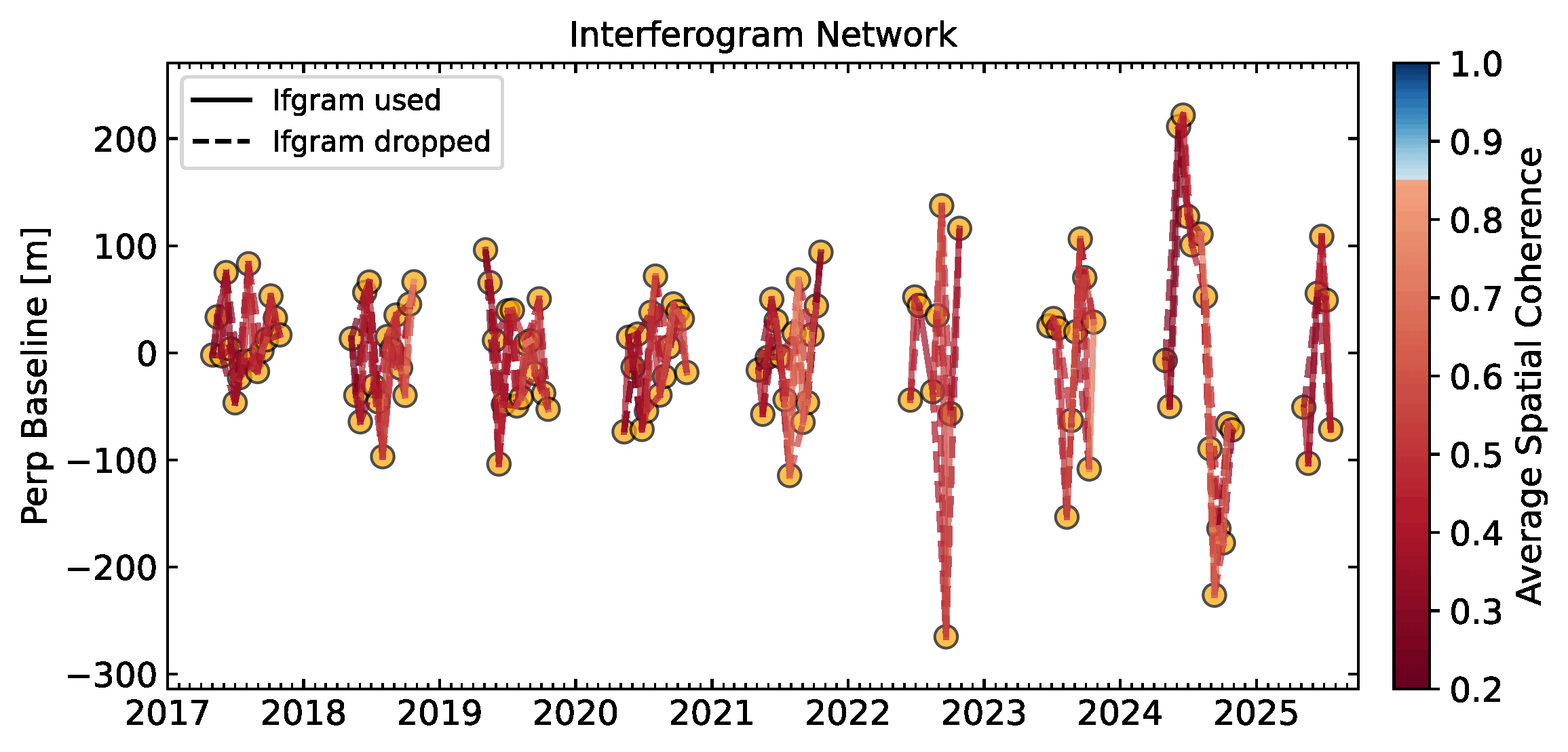
In general, SBAS requires a continuous time series, and in the case of using data only from the snow-free period, this series breaks down into separate groups (see 1b) without direct connections between them – for example, data from 2017 are not connected with 2018, etc. The problem of inversion in SBAS arises when several isolated time series of interferograms are formed, and the connection matrix becomes incomplete. The standard algorithm of the improved SBAS calculates the minimum possible rate of ground displacement during the time interval between snow-free periods. In this case, this displacement was zero. Therefore, similar to [Kakar et al., 2025], it was proposed to fill the gap between snow-free periods with actual displacements obtained for the same time period using GNSS data. For instance, the relative positions of the VODO GNSS station along the LOS were calculated for October 29, 2017, and May 9, 2018, followed by the determination of the displacement between these two dates. To mitigate variations in the estimated relative position, a moving average algorithm was predominantly applied. Linear interpolation was employed only for the PAUJ station due to the absence of GNSS data for the period from August to October 2017. The resulting GNSS-derived displacement for this interval was then incorporated into the SBAS results as the corresponding displacement component. Table 1 below presents the cumulative displacements for GNSS stations during periods not covered by the SBAS measurements. It is worth noting that a similar approach in [Kakar et al., 2025] was used to integrate ENVISAT and Sentinel-1 interferometric data into a single time series, bridging a 5-year gap between the two datasets.
Then, to estimate vertical displacements and displacements along the west-east direction, we used an approach proposed in [Babayantz et al., 2023; Fuhrmann and Garthwaite, 2019] involving data from the ascending and descending orbits. Here, as in [Babayantz et al., 2023], we assume that the northern component of the displacements does not exceed the displacements in other directions. A detailed description of this approach is presented in [Babayantz et al., 2023] and is therefore not described here.
Figure 2 shows the result without accounting for displacements between snow-free periods. It is noteworthy that, despite the numerous white spots, a certain difference in the velocities (colors) of the western and eastern parts is visually noticeable in 1a. However, as for vertical displacements in 1b, the spatial distribution of displacements is more heterogeneous. Therefore, for more accurate identification of areas with similar geodynamics, it is necessary to consider these displacements as a whole. The arrows in Figures 2 and 3 indicate the directions of horizontal displacements of GNSS stations over the entire period under consideration.
| No SBAS data periods | Cumulative GNSS displacements, mm | ||
| Start | End | PAUJ | VODO |
| 2017-10-29 | 2018-05-09 | -2.4 | -18.5 |
| 2018-10-24 | 2019-05-04 | -4.8 | -33.7 |
| 2019-10-19 | 2020-05-10 | -7.3 | -54.5 |
| 2020-10-25 | 2021-05-05 | -9.7 | -72.8 |
| 2021-10-20 | 2022-06-17 | -12.7 | -91.0 |
| 2022-10-27 | 2023-06-24 | -15.7 | -107.7 |
| 2023-10-22 | 2024-05-01 | -18.1 | -123.8 |
| 2024-10-28 | 2025-05-08 | -20.5 | -139.8 |
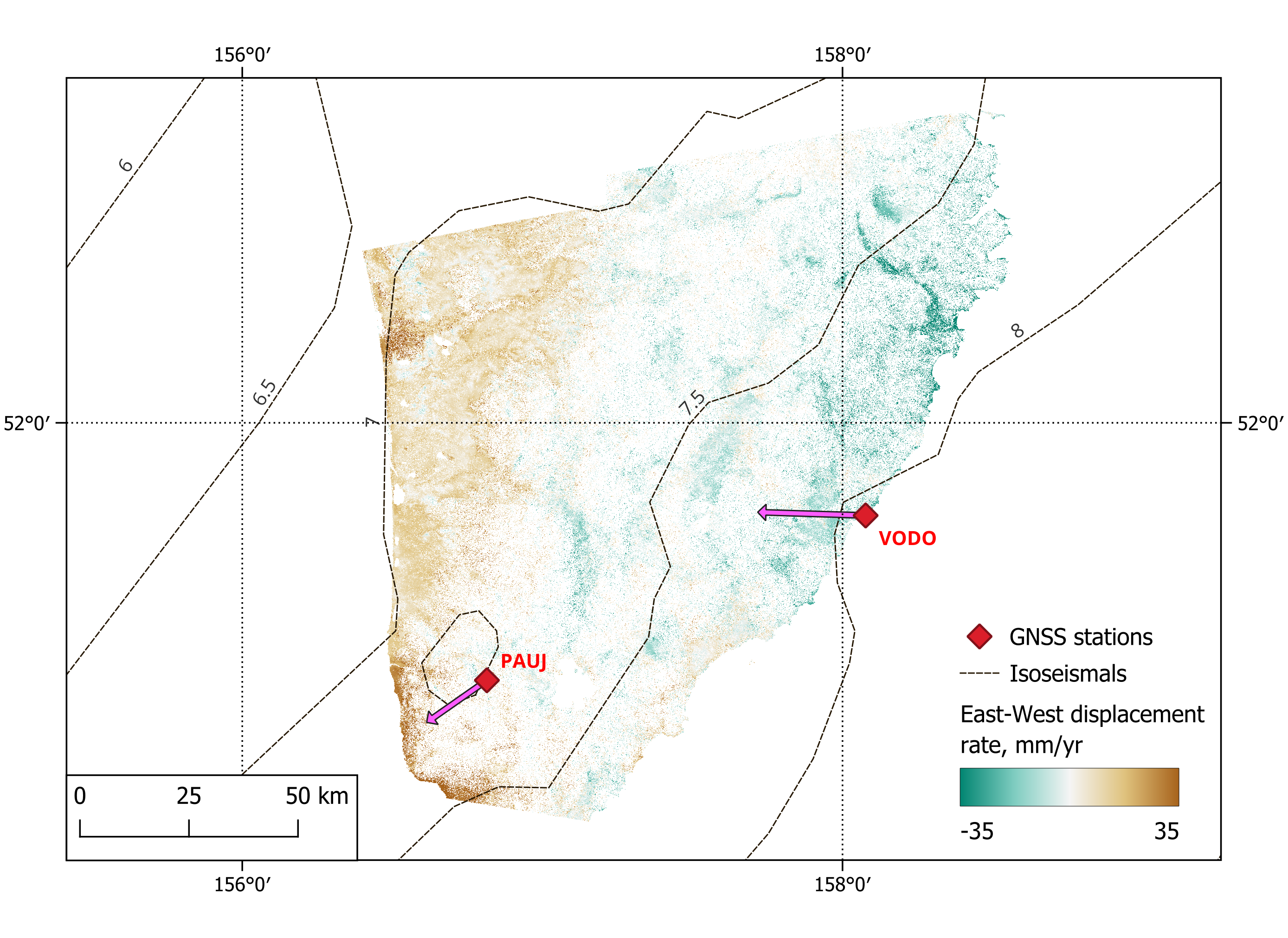
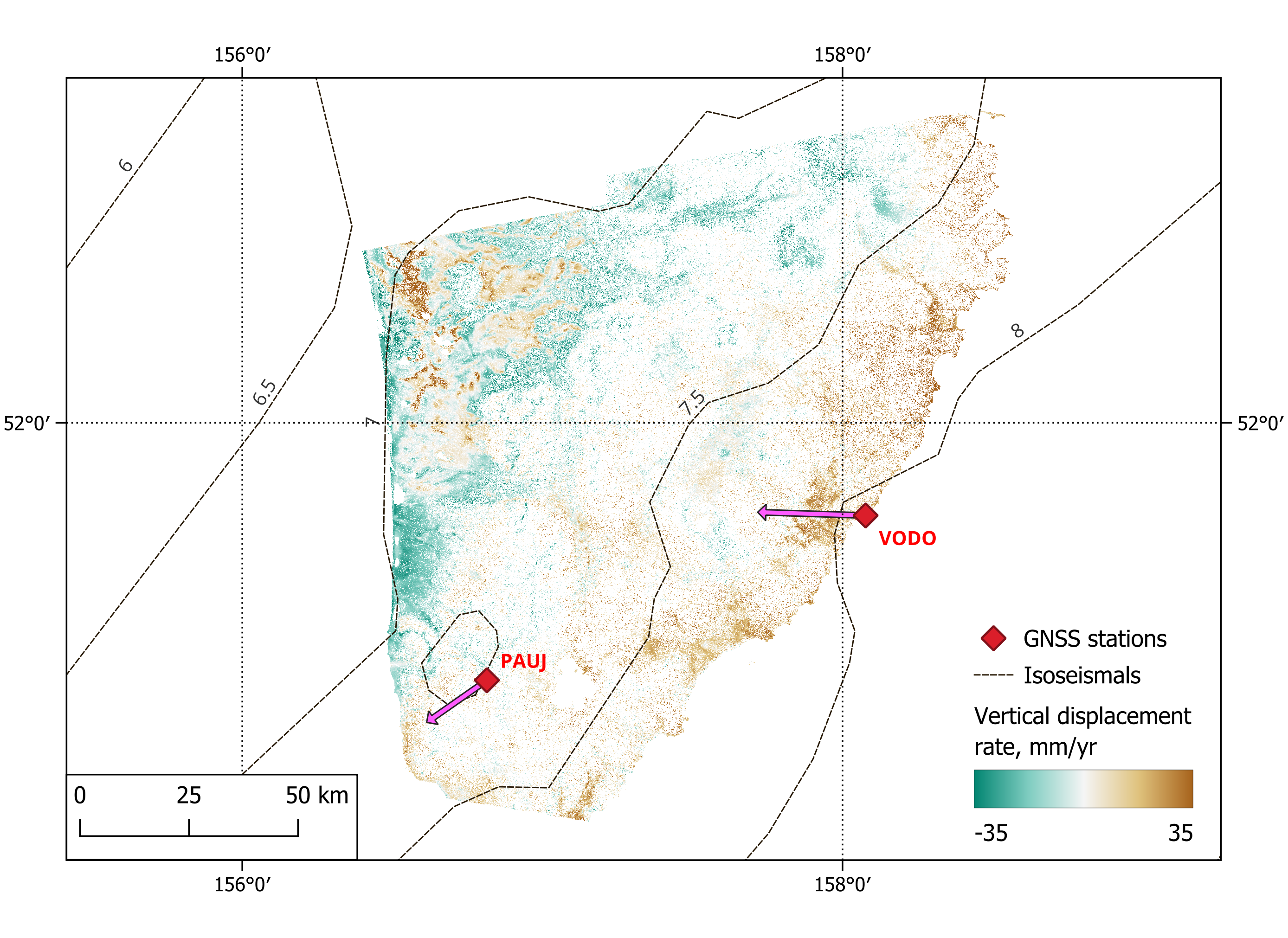
The derived displacement velocity fields were merged to create a two-channel image: the first channel contains the east-west velocity component, and the second channel contains the vertical component. This image, similar to [Bondur et al., 2025], was segmented using the ISODATA clustering method into geoblocks with similar displacement velocity parameters in both directions. With a possible number of clusters ranging from 2 to 15, two clusters were obtained eventually (see Fig. 3). Then we assume that the results of the data cluster analysis represent a true map of the structure of large blocks of area deformations prior to the seismic activity of July 29, 2025. The resulting velocity fields contain significant gaps corresponding to pixels with low coherence and a significant amount of noise in the form of pixels in small groups of 1–3. Therefore, the Sieve operation was run in the ENVI 5.3 software package: 1) Any group of pixels consisting of fewer than 2 pixels is removed; 2) the algorithm considers the neighborhood of each pixel in all eight directions (sides and diagonals), which allows for a more accurate determination of connectivity and the combination of diagonally adjacent pixels into a single group for evaluation. Thus, Sieve acts as a filter, removing single outlier pixels and the smallest, often erroneous, fragments, leaving only statistically significant clusters. Then the Clump operation is run with a window size of \(7 \times 7\) pixels. The algorithm iterates over each remaining pixel after sieving using a sliding window of 7 rows by 7 columns. Within this window, it combines all adjacent pixels of the same class into a single, coherent region. The \(7 \times 7\) window size is relatively large, so it effectively fills gaps and discontinuities within homogeneous areas, smooths boundaries, and combines closely spaced small objects of the same class into larger, continuous arrays.
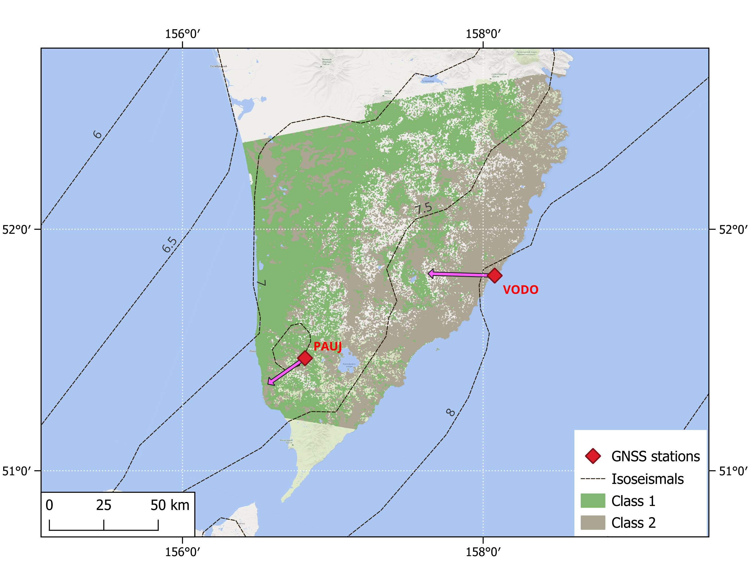
On the one hand, these procedures eliminated numerous blind spots that had not previously been assigned to these two blocks. On the other hand, this significantly increased the spread of values and reduced the accuracy of quantitative estimates of the displacement rates of these main blocks. Nevertheless, the initially “noisy” and speckled displacement velocity fields were transformed into relatively uniform geoblocks: one in the western part of the study area (green) and a narrow band in the eastern part (beige). It should be noted that the space between them is heterogeneous and likely represents a transitional buffer zone (block).
At the same time, it is worth noting features of the spatial structure that, at least, are consistent with contemporary understanding of regional tectonics: the orthogonality of the boundaries between the resulting blocks in the subduction zone, as well as their alignment parallel to the isoseismals presented by the USGS [United States Geological Survey (USGS), 2026].
3 Comparative Analysis of SBAS-Derived Displacements and GNSS Measurements
Let/span>s compare the samples obtained from the line-of-sight displacement velocity field with ground-based data from two GNSS stations, PAUJ and VODO, whose locations are shown in Figure 3. The PAUJ station lies within a transition zone between the eastern and western blocks, where areas exhibit different velocities characteristic of each block. This zone also contains numerous “white spots” (gaps in the data) due to low coherence. The second station, VODO, is located on the eastern block, on the coast of Pacific Ocean. For comparison with the GNSS station data, more than 100 pixels were selected with results obtained using the SBAS method in the vicinity (within a radius of 500–650 m) of each station.
Fig. 4 shows graphs of temporal displacements along the LOS (see green arrow in 1a) for the descending orbit for both stations. The abscissa axis represents the time scale, with the origin corresponding to the first date of the radar survey, and the displacement values (along the ordinate) calculated from this date. The green points in the graphs corresponds to daily GNSS measurements, converted into displacements along the LOS using the formula presented in [Mikhailov et al., 2025]. The red crosses corresponds to SBAS displacements.
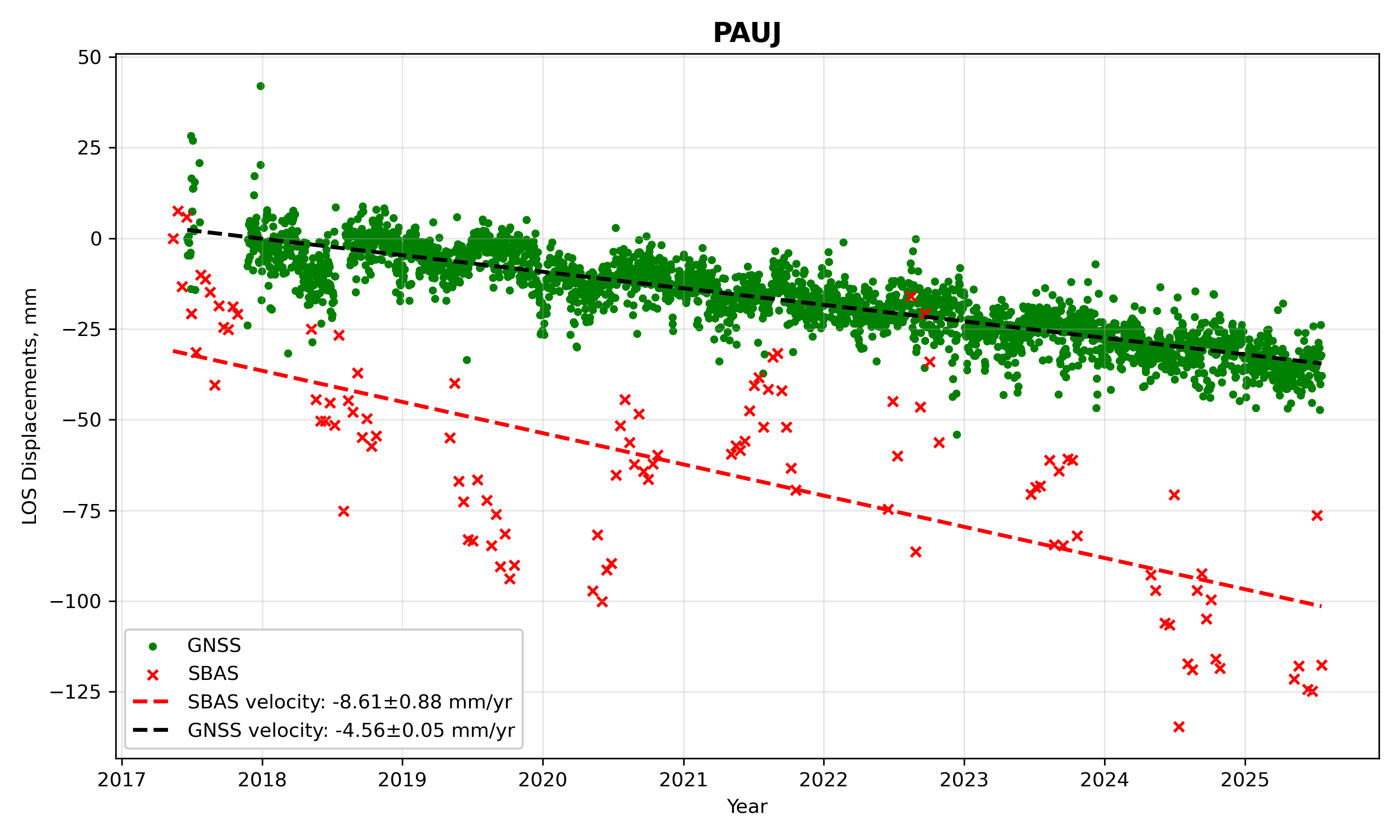
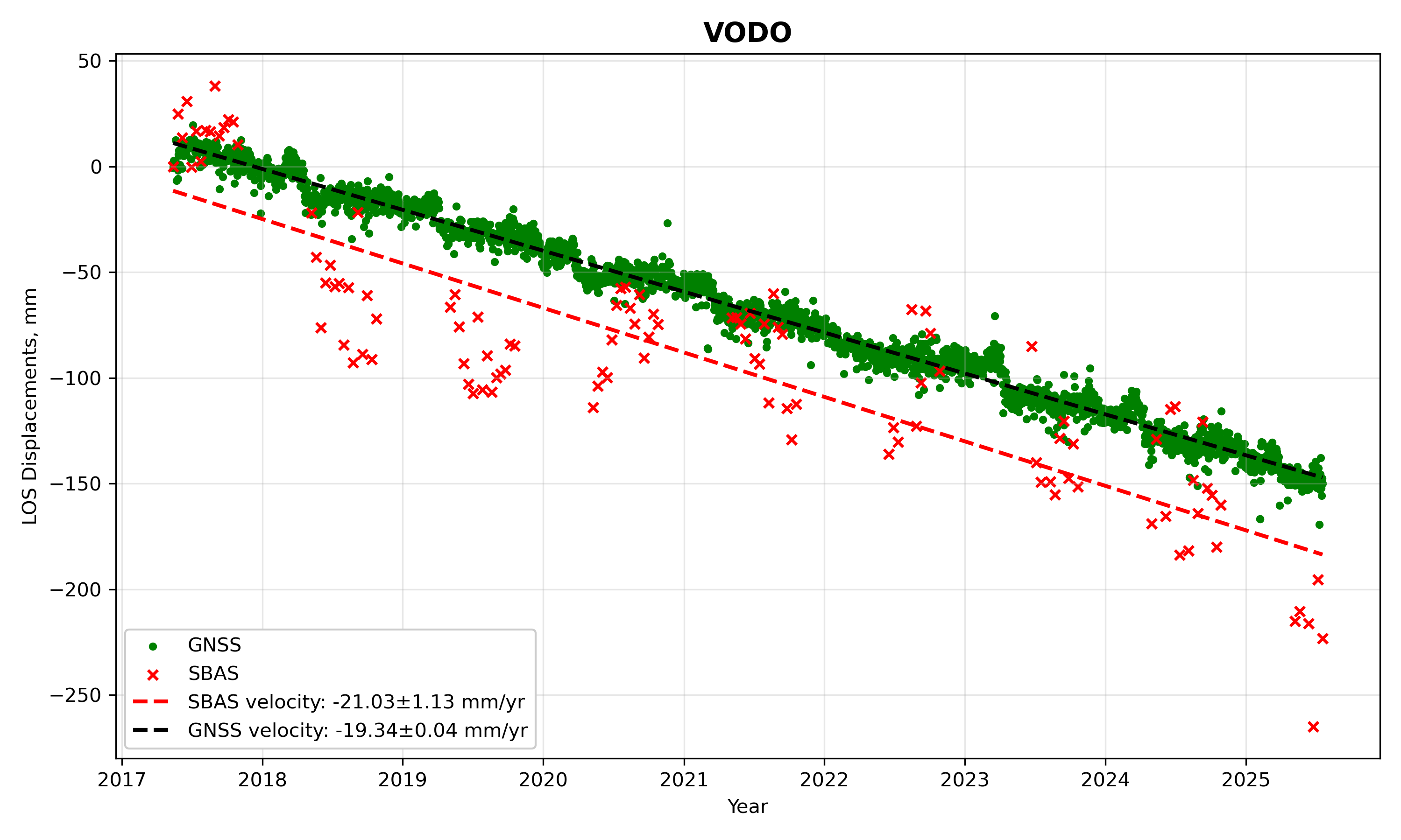
The directions of displacements obtained from SBAS samples are generally consistent with GNSS, so it is proposed to consider that the displacements on the graphs characterize the geodynamics of the corresponding blocks.
However, significant variations in the SBAS values are observed in the graphs. These variations are likely due to the influence of spatiotemporal variations in soil moisture, vegetation, and tropospheric water vapor content on radar interferometric measurements. During the season with less precipitation, soil drying, moisture loss, and a decrease in the height of phase scattering centers in the surface layers manifest themselves in a subsidence of the reflecting surface observed along the line of sight. During this period, tropospheric delays are minimal; however, digital elevation model (DEM) errors or loss of coherence can amplify the effect of displacement away from the satellite. Otherwise, during the wet season with heavy precipitation, soil swelling and the rise of phase scattering centers, associated with increasing permittivity, cause a satellite-directed displacement of the reflecting surface (positive displacements along the LOS in Figure 4).
These patterns are confirmed in recent publications. As shown in [Widhalm et al., 2025], seasonal deformations derived from InSAR data capture spatial variations in soil moisture: areas with higher moisture content exhibit greater uplift due to soil swelling compared to drier locations. Study [Talgarbayeva et al., 2025] documented uplift of over 30 mm due to swelling of saturated soil, while [Westerhoff and Steyn-Ross, 2020] presented evidence that small temporal differences in soil and vegetation moisture can have a relatively large influence on microwave radiation phase perturbations, with vegetation dominating this influence. Based on this, [Westerhoff and Steyn-Ross, 2020] concluded that differences in soil and vegetation moisture can indicate false displacement in satellite radar interferometry data. Thus, the observed isolated anomalies in the displacements obtained by the SBAS method should be mitigated by considering the trend.
Thus, linear trends from Fig. 4 indicate that the VODO displacement rate \(-19.3\)(GNSS) / \(-21.0\)(SBAS) mm/year along LOS and accordingly assume along the entire eastern block, exceeds the PAUJ rate \(-4.6\)(GNSS) / \(-8.6\)(SBAS) mm/year by several times. The latter station, as noted above, is located in some transition zone but could also possibly be classified as part of the western block. This latter conclusion requires further research.
4 Conclusion
As a result of the conducted study, the task of identifying and assessing the dynamics of large geoblocks in the southern part of Kamchatka was solved based on the analysis of interseismic deformations that preceded the powerful seismic activity on July 29, 2025.
The primary research method was an improved SBAS radar interferometry method implemented in the MintPy software package. To overcome specific regional challenges – heavy snow cover [Dagurov et al., 2020; Tananaev et al., 2025] and challenging atmospheric conditions – a comprehensive methodology was employed. This included data analysis exclusively during the snow-free period (May–October) with a high coherence threshold (0.75) and synergistic merging of SBAS time series with GNSS measurements to fill gaps between seasons, similar to the approach described in the literature. Atmospheric delay correction was performed, taking into account the recommendations [Volkova et al., 2025] regarding the need for a thorough analysis of the effect of the corrections applied.
The processing of long-term Sentinel-1 data (2017–2025) and subsequent decomposition of displacement velocities into vertical and horizontal (west–east) components allowed us to obtain deformation fields. ISODATA clustering of these fields revealed that the territory was divided into two large blocks with different geodynamics western and eastern, separated by a transition zone. The spatial configuration of the identified blocks – their orthogonality to the subduction zone and parallelism to the isoseismals of the 2025 earthquake – is consistent with modern concepts of regional tectonics. For example, work [Shestakov et al., 2024] indicates 1) movements in the entire study region as a whole (the Kuril–Kamchatka Trench) are oriented approximately orthogonally to the subduction zone boundary and 2) an increase in the rate of subduction of the Pacific lithospheric plate or part of it under the overlying North American plate.
A comparative analysis with data from the PAUJ and VODO GNSS stations, located in the transition zone and eastern block, respectively, confirmed the general direction of the trends obtained using the SBAS method and GNSS measurements. Moreover, the observed variations in SBAS values, according to the literature, can be explained by the influence of seasonal changes in soil moisture and vegetation [Talgarbayeva et al., 2025; Westerhoff and Steyn-Ross, 2020; Widhalm et al., 2025]. Linear trends showed that the displacement rate of the eastern block (VODO station, \(-19.3\) mm/year) is several times higher than the rate in the western block/tranzition zone (PAUJ station, \(-4.6\) mm/year).
Thus, the developed method, combining the advantages of SBAS InSAR (dense spatial coverage) and GNSS (high temporal accuracy and continuity), made it possible to identify a block structure characterizing the geodynamics during the study period in the complex natural conditions of Kamchatka. The resulting map of interseismic deformations and quantitative estimates of the displacement rates of key geoblocks will improve our understanding of the spatial heterogeneity of the lithosphere/span>s stress-strain state prior to major earthquakes. These results serve as the basis for further research on seismic hazard assessment and the construction of physical models for the preparation of megaquakes in subduction zones.
Acknowledgments. The research was carried out in the frameworks of the state assignments of ISR “AEROCOSMOS”, Institute of Physical Materials Science of SB RAS, and Kamchatka Branch of the Geophysical Survey of RAS.
1. Babayantz I. P., Mikhailov V. O., Timoshkina E. P., et al. On the accuracy of the vertical and eastern components of the Earth’s surface displacements calculated from SAR images obtained from two orbits // Sovremennye problemy distantsionnogo zondirovaniya Zemli iz kosmosa. — 2023. — Vol. 20, no. 2. — P. 135–143. — https://doi.org/10.21046/2070-7401-2023-20-2-135-143
2. Berardino P., Fornaro G., Lanari R., et al. A new algorithm for surface deformation monitoring based on small baseline differential SAR interferograms // IEEE Transactions on Geoscience and Remote Sensing. — 2002. — Vol. 40, no. 11. — P. 2375–2383. — https://doi.org/10.1109/TGRS.2002.803792
3. Bondur V. G., Chimitdorzhiev T. N. and Dmitriev A. V. The Induced Seismicity Effect in Morocco Caused by a Reduced Aquifers Volume according to Stacking-InSAR Method and Gravimetric Data // Doklady Earth Sciences. — 2024. — Vol. 517, no. 1. — P. 1269–1275. — https://doi.org/10.1134/S1028334X24601809
4. Bondur V. G., Chimitdorzhiev T. N. and Dmitriev A. V. The Geodynamics before and after the February 6, 2023 Earthquake Doublet in Turkey According to Satellite Radar Interferometry Data // Doklady Earth Sciences. — 2025. — Vol. 523, no. 1. — https://doi.org/10.1134/s1028334x25606558
5. Bondur V. G., Chimitdorzhiev T. N., Tubanov Ts. A., et al. Analysis of the Block-Fault Structure Dynamics in the Area of Earthquakes in 2008 and 2020 near Southern Lake Baikal by the Methods of Satellite Radiointerferometry // Doklady Earth Sciences. — 2021. — Vol. 499, no. 2. — P. 648–653. — https://doi.org/10.1134/S1028334X21080031
6. Chen S., Ma M., Ma Yo., et al. Three-dimensional deformation monitoring of San Francisco Bay based on GNSS-InSAR data // Advances in Space Research. — 2025. — Vol. 75, no. 1. — P. 451–464. — https://doi.org/10.1016/j.asr.2024.09.057
7. Chimitdorzhiev T. N., Dmitriev A. V., Kirbizhekova I. I., et al. Preliminary results of radar interferometry of the area of the Kamchatka earthquake of July 29, 2025 // Proceedings of 23 International Conference "Current Problems in Remote Sensing of the Earth from Space", Moscow, Space Research Institute, November 10-14, 2025. — Moscow : Space Research Institute Publ., 2025. — https://doi.org/10.21046/23DZZconf-2025a — (In Russian).
8. Dagurov P. N., Chimitdorzhiev T. N., Dmitriev A. V., et al. Estimation of snow water equivalent from L-band radar interferometry: simulation and experiment // International Journal of Remote Sensing. — 2020. — Vol. 41, no. 24. — P. 9328–9359. — https://doi.org/10.1080/01431161.2020.1798551
9. Ferretti A., Prati C. and Rocca F. Permanent scatterers in SAR interferometry // IEEE Transactions on Geoscience and Remote Sensing. — 2001. — Vol. 39, no. 1. — P. 8–20. — https://doi.org/10.1109/36.898661
10. Fuhrmann T. and Garthwaite M. C. Resolving Three-Dimensional Surface Motion with InSAR: Constraints from MultiGeometry Data Fusion // Remote Sensing. — 2019. — Vol. 11, no. 3. — P. 241. — https://doi.org/10.3390/rs11030241
11. Guo N., Wu Y. and Su G. Analysis of the fault slip, creep, and coupling characteristics of the Maomaoshan-LaohushanHaiyuan Fault using InSAR and GNSS measurements // Tectonophysics. — 2023. — Vol. 863. — P. 229988. — https://doi.org/10.1016/j.tecto.2023.229988
12. Hogenson K., Kristenson H., Kennedy J., et al. Hybrid Pluggable Processing Pipeline (HyP3): A cloud-native infrastructure for generic processing of SAR data. — 2025. — https://doi.org/10.5281/zenodo.15724929
13. Kakar N., Zhao Ch., Li G., et al. Spatio-temporal analysis of subsiding districts in Balochistan, Pakistan using Multi-Sensor SBAS InSAR and GNSS // Natural Hazards. — 2025. — Vol. 121, no. 9. — P. 10553–10581. — https://doi.org/10.1007/s11069-025-07226-y
14. Li Y., Zuo X., Xiong P., et al. Deformation monitoring and analysis of Kunyang phosphate mine fusion with InSAR and GPS measurements // Advances in Space Research. — 2022. — Vol. 69, no. 7. — P. 2637–2658. — https://doi.org/10.1016/j.asr.2021.12.051
15. Mikhailov V. O., Konvisar A. M., Smirnov V. B., et al. The Rupture Surface Model of the July 29, 2025 Mw 8.8 Kamchatka Earthquake Based on Satellite Geodesy and Interferometry Data // Doklady Earth Sciences. — 2025. — Vol. 525, no. 2. — https://doi.org/10.1134/S1028334X25608752
16. Shestakov N. V., Nechaev G. V., Titkov N. N., et al. GNSS-Based Modeling and Study of Postseismic Crustal Movement of the May 24, 2013, MW 8.3 Sea of Okhotsk Deep-Focus Earthquake // Geodynamics & Tectonophysics. — 2024. — Vol. 15, no. 3. — P. 0761. — https://doi.org/10.5800/gt-2024-15-3-0761 — (In Russian).
17. Talgarbayeva D., Vilyaev A., Dedova T., et al. InSAR monitoring of dam deformations in a seismically active region of Kazakhstan for identifying precursors of failure // Frontiers in Earth Science. — 2025. — Vol. 13. — https://doi.org/10.3389/feart.2025.1638088
18. Tananaev N. I., Timofeev M. A. and Zakharov M. I. Snow cover of Kamchatka: Actual features and projections of change // GEOSYSTEMS OF NORTH-EAST ASIA: natural, social and economic systems. — Vladivostok : POI FEB RAS Publ, 2025. — P. 188–192. — https://doi.org/10.35735/9785605278788_188 — (In Russian).
19. Tao Q., Liu R., Li X., et al. A method for monitoring three dimensional surface deformation in mining areas combining SBAS-InSAR, GNSS and probability integral method // Scientific Reports. — 2025. — Vol. 15, no. 1. — https://doi.org/10.1038/s41598-025-87087-4
20. United States Geological Survey (USGS). M 8.8 - 2025 Kamchatka Peninsula, Russia Earthquake. — URL: https://earthquake.usgs.gov/earthquakes/eventpage/us6000qw60 (visited on 02/06/2026).
21. Volkova M. S., Mikhailov V. O. and Osmanov R. S. Comparison of Atmospheric Corrections Models to Satellite Interferometry Data on Kamchatka Region // Earth Research from Space. — 2025. — No. 3. — P. 13–25. — https://doi.org/10.7868/s3034540525030027 — (In Russian).
22. Westerhoff R. and Steyn-Ross M. Explanation of InSAR Phase Disturbances by Seasonal Characteristics of Soil and Vegetation // Remote Sensing. — 2020. — Vol. 12, no. 18. — P. 3029. — https://doi.org/10.3390/rs12183029
23. Widhalm B., Bartsch A., Strozzi T., et al. InSAR-derived seasonal subsidence reflects spatial soil moisture patterns in Arctic lowland permafrost regions // The Cryosphere. — 2025. — Vol. 19, no. 3. — P. 1103–1133. — https://doi.org/10.5194/tc-19-1103-2025
24. Yunjun Z., Fattahi H. and Amelung F. Small baseline InSAR time series analysis: Unwrapping error correction and noise reduction // Computers & Geosciences. — 2019. — Vol. 133. — P. 104331. — https://doi.org/10.1016/j.cageo.2019.104331
25. Zakharov A. and Zakharova L. An Influence of Snow Covers on the Radar Interferometry Observations of Industrial Infrastructure: Norilsk Thermal Power Plant Case // Remote Sensing. — 2023. — Vol. 15, no. 3. — P. 654. — https://doi.org/10.3390/rs15030654
26. Zhang L., Dai K., Deng J., et al. Identifying Potential Landslides by Stacking-InSAR in Southwestern China and Its Performance Comparison with SBAS-InSAR // Remote Sensing. — 2021. — Vol. 13, no. 18. — P. 3662. — https://doi.org/10.3390/rs13183662